Magnetohydrodynamic (MHD) Propulsion Boat - Presentation, Analysis And Interpretation of Data

This is Chapter 3 of the investigatory project entitled "Speed of a Magnetohydrodynamic Propulsion Boat as a Function of Salt Concentration" submitted to Science and Mathematics Education Department (SMED) of University of San Carlos. This lays down the presentation, analysis and interpretation of data.
You may need to read the other chapters to see the study as a whole. Below are the links:
CHANNEL WIDTH OPTIMIZATION
Shown below is the data gathered from the measurements of the magnetic field strength between the magnets used in the boat channel. The averages of the field strengths for every magnet separation (W) are also shown.

The averaging of those magnetic fields may seem invalid, but it provides an acceptable estimation. The entire process of width optimization was not concerned with finding the distance separation with the greatest magnetic field (in this case it is clear that making the separation smallest would give the higher field), but rather on finding which would provide a higher net total of electromotive force. Indeed 7 mm has higher magnetic field between them compared to 19 mm, but by virtue of being the channel narrow, only a small amount of solution passes through it, and thus the propulsion is weak. Increasing the channel width further from 19mm would allow more water to pass through, but at the cost of lowered magnetic field strength, and thus lowered propulsion.
The magnetic field strengths (B) were graphed against the distance from the north pole of one magnet (y) for every separation (W ).

As shown in the graph, the magnetic field strength decreases as the distance from the north pole increases, and increases back again as it becomes closer to the south pole of the other magnet. This is due to the inverse square relationship between magnetic field strength and distance. It can also be seen that the magnetic field strength of the first array of magnets which served as the north pole was stronger than the other. If they have had the same strength, the graph would equal tips of the parabolic curve.
To be able to find the optimum channel width, the average magnetic field was graphed against the magnet separation (W ).

Using Microsoft Excel, the equation of the trend line of the above graph, which gives the magnetic strength of the array of magnets used in the experiment as a function of separation, was found to be:

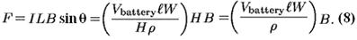
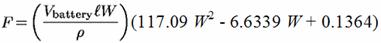
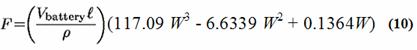
As shown in the graph, the average magnetic field decreased as the distance between the magnets increased. Inserting this equation of the trend line to Eq. 8 (derived in the Theoretical Background) yields an empirical force function that is proportional to a cubic function of W:

The results show that an optimum does indeed exist. As the magnet separation increases from zero, the force also increases. The result was that the maximum was reached between 19 and 20 mm, after which the force decreases due to the diminishing magnetic field.
The exact value of this maximum point can be determined by applying the first derivative to the equation of the above graph’s trend line. The equation of the curve fit is:
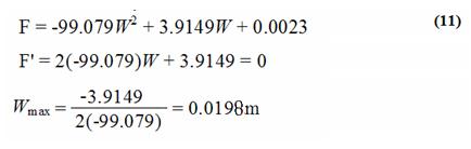
The MHD boat water channel width (W) in the present study was therefore chosen to be 1.98 cm. These results were specific to the magnets chosen. If another pair of magnets was to be used, width optimization should be done again.
RELATIONSHIP BETWEEN CONCENTRATION AND BOAT SPEED
Shown below is the data gathered from the research set-up.

The mass of the NaCl dissolved for every solution was measured by a weighing scale. The volume was measured accurately using a volumetric flask. The concentration was determined by dividing the mass of dissolved salt in kilograms by the volume of water in liters. The data for the three trials for the time of travel were taken from the digital counter. The average of the three data for each set was also determined. The distance traveled during the time interval measured was equal to the diameter of the “flag” as measured by a Vernier caliper. The speed was calculated by dividing the distance traveled in centimeters by the time of travel in seconds.
The relationship between the speed of the MHD boat and the concentration of the salt solution on which it runs on can be easily seen if we graph the data found in Table 2, as shown below:

As is shown by the trend line (red), there was a parabolic relationship between the speed of the MHD boat and salt concentration. The graph has a coefficient of correlation r2 of 0.9655. This means that 96.55% of the data gathered falls within this curve. As the concentration increases from zero, the speed that the boat attained increases. However, when the concentration reaches a certain point, the increase in speed stops. If the concentration is increased further, the maximum speed attainable by the boat decreases.
The concentration on which the boat travels fastest was determined by applying the first derivative to the equation of the above graph’s trend line. The equation of the trend line was found to be:

where S is the speed of the boat in cm/s while C in the salt concentration in kg/L. Getting the first derivative and equating it to zero, we have:

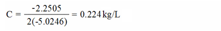
The boat was able to attain its maximum speed at a salt concentration of 0.224 kg/L. This concentration is the same as dissolving 3.14 kilograms of salt in 14 liters of water. For a point of reference, since 35 grams of NaCl is needed to saturate 100 mL of water, it requires 4.90 kilograms to completely saturate 14 liters of distilled water.


