Methods Of Analysis To Determine Stresses In Inflatable Dam Models

Two numerical methods were employed to analyze the stresses in inflatable dam models. The first method was based on Harrison's finite element approach and the second was based on Parbery's continuous approach.

The two analytical methods were written into computer programmes which calculate the theoretical profile shape of an inflatable dam. The profile shape measured experimentally were compared with those obtained from the theoretical calculations.

Assumptions

The finite element method for analyzing an inflatable dam was carried out on the basis of three assumptions. The first assumption was to regard the behaviour of the three dimensional structure as being represented reasonably by the behaviour of a two dimensional section of unit width. The second assumption was to consider the perimeter of the section as composed of a finite number of small elements which could be treated as straight. The third assumption was to assume that loads acting on each length of any element caused by water and air pressures could be considered as acting as concentrated loads at the extremities os such an element.

Fig. (6) shows the forces acting on an inflatable dam due to the upstream, downstream and inflation heads.

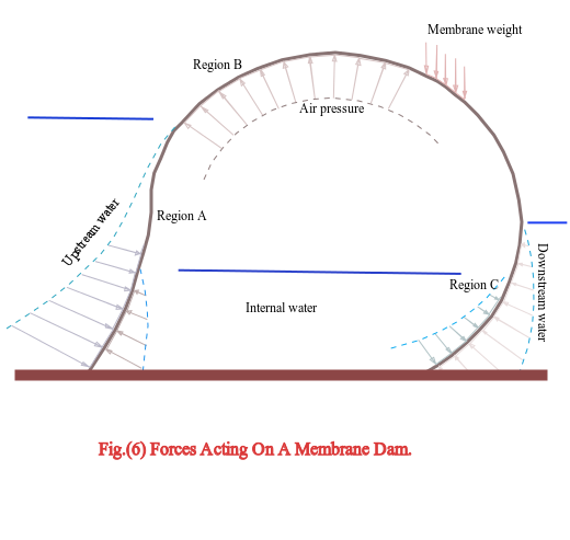
Along the profile curve of the dam, the membrane is divided into an upstream region, an atmosphere region and a downstream region. The regions are denoted as region A, B and respectively in Fig. (6).

An element of the dam membrane in region A has external forces acting on it due to the upstream and inflation heads. The inflation head can arise from air or water pressure or a combination of both.

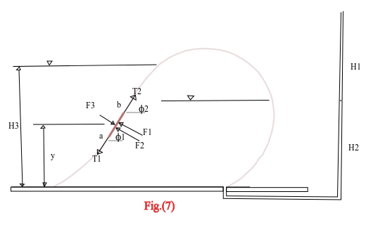
Fig. (7) shows the various measured parameters of a loaded inflatable dam and also an element 'ab' in region A subjected to the various forces.

The notations used in Fig. (7) are defined as follows;

• H₁ = internal air pressure head.
• H₂ = internal water pressure head.
• H₃ = upstream head.
• H₄ = downstream head.
• F₁ = force on element due to internal air pressure.
• F₂ = force on element due to internal water pressure.
• F₃ = force on element due to downstream head.
• T₁ = tension in element at end a.
• T₂ = tension in element at end b.
• Q₁ = inclination of T₁.
• Q₂ = inclination of T₂.
• WT = weight of element.

The internal air pressure inside the dam is constant, thus the forces on the element due the air pressure is

F₁ = H₁ . ρ . g . EL

where EL is the length of the element, p is the density of water and g is the acceleration due to gravity.

The forces on the element contributed by the internal water pressure and the upstream head are respectively,

• F₂ = ( H₂ - y ) ρ . g . EL
• F₃ = ( H₃ - y ) ρ . g . EL

where y is the average elevation of the element above the dam base.

The element is in equilibrium, so solving the forces horizontally and vertically gives the following equations,

Eq.(1): TX = ( F₁ + F₂ + F₃ ).sin Ø₁ + T₁.cos Ø₁

Eq.(2): TY = ( F₃ - F₂ - F₁ ).cos Ø₁ + T₁.sin Ø₁ + WT

where TX and TY are the horizontal and vertical component of T₂.

In region B there is no external load from outside the dam, so F = 0 on any element in this region. The value of F₂ also becomes zero when the elevation of the element is above H₂.

Beyond the crest of the dam, the weight WT of an element is in the same direction as that of TY. Therefore, the sign of WT is negative in equation ( 2 ) when considering an element on the downstream face.

The outside external force in region C comes from the downstream head. The force F3 on an element in this region is

F₃ = ( H₄ - y ).ρ.g.EL

For the water inflated dam, the value of F₁ is zero while for the air inflated dam F₂ is zero.

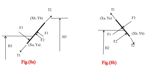
The forces F₁, F₂ and F₃ calculated above are for any element which is completely subjected to the loading pressures over its whole length. In the computation however, there occurred cases when elements were partially loaded. Two examples of such a case are as shown in Fig. (8a) and Fig. (8b).

In Fig.(8a), F₃ = ( H₃ - Ya )² . ρ . g . EL / ( 2 ( Yb - Ya ))

In Fig.(8b), F₂ = ( H₂ - Yb )² . ρ . g . EL / ( 2 ( Yb - Ya ))

The heads H₁, H₂, H₃ and H₄ were measured directly, thus allowing the forces F₁, F₂ and F₃ acting on an element at an elevation Y above the dam base to be calculated. The weight WT of the element was found since the weight per unit area of the membrane was known. This leaves on the right hand sides of equations ( 1 ) and ( 2 ), T₁ and Ø1 as variables.

In the analysis, the tension T₁ and the slope Ø₁ of the first element at the upstream fixture were assumed to have certain trial values. Thus, the values of TX and TY could be calculated in terms of those trial values.

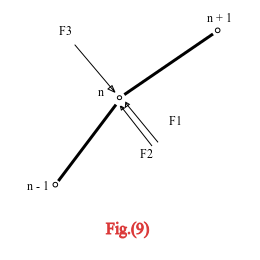
In Fig. (9), it can seen that the external forces F₁, F₂ and F₃ acting on node n are the sums of those acting on the upper half and the lower half of the elements n and n+1 respectively. However, the coordinates of node n+1 was not known.

For the first estimation of the position of node n+1, it was assumed the forces F₁, F₂ and F₃ on node n to be equal to those acting on the element n. Using equations ( 1 ) and ( 2 ), the values of TX and TY were found, and thus the value of T₂. The inclination of the element n+1 lies in line with the line of action of the tension T₂. The inclination and the tension are respectively expressed as follows;

• Q₂ = tan -1 ( TY / TX )
• T₂ = TX² + TY²

Thus, the coordinates of node n+1 are;

X_n+1 = X_n + EL ( 1 + T₂ / ( t . E )) cos Q2

Y_n+1 = Y_n + EL ( 1 + T₂ / ( t . E )) sin Q2

where t and E are the thickness and elastic modulus of the membrane material which accounts for the extensibility of the element due to the tension T2.

The forces on the element n + 1 where then calculated in a similar manner. The average external forces acting on element n and n + 1 were taken to act on node n. A better estimation of the position of node n + 1 was then re-calculated.

The procedure was repeated around the curved perimeter until the final node was computed. Solutions were achieved if the coordinates of the final node coincide with the known position of the downstream fixture.

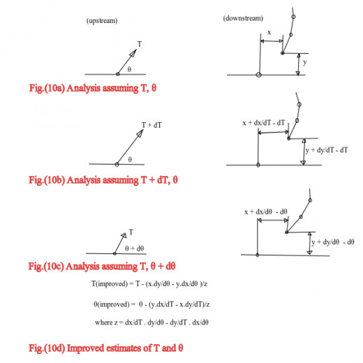
For a pair of assumed initial values of tension and slope ( T, O ), in the first element there would be a miss-closure between the computed final node and the downstream fixture. The Newton Method of iteration was used to adjust these assumed initial values so that the computed coordinates of the final node would coincide with the known position of the downstream fixture.

In Fig. (10a), it can be seen that miss closures X and Y do result when arbitrary values T and O are assumed for the first element. When the analysis is repeated, with T increased by a small amount as in Fig. (10b), different miss closure components will be calculated from which the rate of change of X and Y with respect to T may be approximately evaluated. Similar rate of change of X and Y with respect to O may be computed by a third analysis as shown in Fig. (10c). Improved values of tension and slope are the determined numerically from the Newton expression shown in Fig. (10d).

In the analysis, the iteration procedure was repeated until the miss closures were reduced to negligible values.

Derivation of the differential equations of equilibrium.

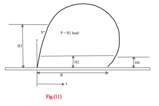
Fig. (11) defines the various parts of the two dimensional dam model.

The upstream fixture is the origin of the x-y coordinates system. S* is the distance along the curved perimeter in the loaded state. The membrane is assumed to weigh w per unit area and to obey an elastic relationship of the form ɛ = g(ρ), where ɛ and ρ are the strain and stress in the membrane respectively.

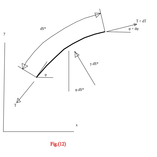
Fig. (12) shows the loads acting on an elemental strip dS* of unit width, where p is the resultant internal pressure and T is the tension per unit width.

Summing the forces in Fig. (12) in the tangential direction gives

T + dS*.W.sin Ø = (T + dT) cos Ø

where O is the inclination of the elemental strip to the positive x-direction.

As dS* -> 0, dØ -> 0, giving Ø = 1.

Therefore, the equation above can be written as

Eq. (3): dT/dS* = w.sin Ø

In the normal direction, the forces can be expressed in the form

T = rP

where P = p - w.cos Ø

and r = dS*/dØ

Eq.(4): i.e. T = -dS*/dØ (p - w.cos Ø)

The sign convention adopted for the radius of curvature is that the normal convex shape of the dam corresponds to positive curvature.

In addition, from Fig. (12),

Eq.(5): dx/dS* = cos Ø

and Eq.(6): dy/dS* = sin Ø

It is convenient to use the distance S along the un-stretched membrane as the independent variable. The relationship between S and S* is as follows;

Eq.(7): dS*/dS = 1 + g(ρ) = f(ρ)

The Cartesian origin is chosen so that x(O) = 0 and y(O) = 0.

Substituting equation (6) into Eq.(3) gives;

dT/dS* = w.dy/dS*

or dT = w.dy

As dT -> 0 and dy -> 0,

dT = w.dy

Integrating, gives

Eq.(8): T = To + w.y

where To = T(0).

Substituting Eq.(8) into Eq.(4) gives

Eq.(9): dØ/dS* = -1.(p - w.cos Ø)/(To + w.y)

By eliminating dS* using Eq.(7), the Eq.(9), (5) and (6) are rewritten as follows respectively;

Eq.(10): dØ/dS = f(ρ)(p - w.cos Ø)/(To + wy)

Eq.(11): dx/dS = f(ρ) cos Ø , and

Eq.(12): dy/dS = f(ρ) sin Ø

The differential equations (10), (11) and (12) together with the following boundary conditions

Eq.(13): x(0) = 0

Eq.(14): y(0) = 0

Eq.(15): x(L) = B

and Eq.(16): y(L) = 0

define the equilibrium shape of the inflatable dam. L and B are the un-stretched perimeter length and the base length respectively.

In the analysis, the differential equations were solved by employing a fourth order Runge-Kutta method. The differential equations are denoted as follows;

f₁(y,Ø) =dØ/dS

f₂(Ø) = dx/dS

f₃(Ø) = dy/dS

If the coordinates of an arbitrary point n on the membrane are (x_n, y_n) and the inclination of a small strip dS at that point is Ø_n, then using the Runge-Kutta method the following the following parameters are defined.

k₁ = dS.f₁(y_n, Ø_n)

l₁ = dS.f₂(Ø_n)

m₁ = dS.f₃(Ø_n)

k₂ = dS.f₁(y_n + m₁/2, Ø_n + k₁/2)

l₂ = dS.f₂(Ø_n + k₁/2)

m₂ = dS.f₃(Ø_n + k₁/2)

k₃ = dS.f₁(yn + m₂/2, Ø_n + k₂/2)

l₃ = dS.f₂(Ø_n + k₂/2)

m₃ = dS.f₃(Ø_n + k₂/2)

k₄ = dS.f₁(y_n + m₃, Ø_n + k₃)

l₄ = dS.f₂(Ø_n + k₃)

m₄ = dS.f₃(Ø_n + k₃)

The inclination of the proceeding small strip and the coordinates of the proceeding point on the membrane are given by the expressions below;

Eq.(17): Ø_n+1 = Ø_n + (k₁ + 2.k₂ + 2.k₃ + k₄)/6

Eq.(18): x_n+1 = x_n + (l₁ + 2.l₂ + 2.l₃ + l₄)/6

Eq.(19): y_n+1 = y_n + (m₁ + 2.m₂ + 2.m₃ + m₄)/6

The shape of the dam profile was calculated using the equations (17), (18) and (19) with estimates of Ø(0) and T(0) which were then refined using the Newton method of iteration as explained in section above.

For an inextensible membrane the value of f(ρ) is equal to 1. Considering the extensibility, the value of f(ρ) will be greater than 1 and it will depend on the tension T, the thickness t and the elastic modulus E of the membrane material. In the analysis, f(ρ) was incorporated into the value of dS which was used as the step length in the Runge-Kutta method of integration, thus taking extensibility into account.

The resultant pressure p acting on an element strip was determined in a similar manner to that used in the determination of the forces on an element explained in section above. In the continuous analysis, the resultant pressure p on one elemental strip was incorporated in the calculation of the coordinates of a point, while in the finite element analysis, the average forces on two consecutive elemental strips were used to calculate the coordinates of a point of the profile shape.

The initial trial values of tension and slope were made by assuming the loaded shape of an inflatable dam profile to be circular. The pressure difference between both sides of the membrane was assumed to be constant, and thus the equation T = rP* was used to calculate the initial guessed tension, where T is the tension in the membrane, r is the radius of curvature and P is the pressure difference between the membrane surfaces.

Fig.(13) shows the idealized profile shape of an inflatable dam.

(a) For an air inflated dam, the inflation pressure is constant everywhere inside the dam, so that the pressure difference

P = inflation air pressure = H₁.p.g

(b) For water inflated dam, the inflation pressure varies with the height of the dam. The pressure at the mid-height of the dam was used in the calculation of the tension, i.e.

P = (H₂ - r).ρ.g

where H2 is the inflation head measured at the bottom of the dam.

In the estimation of the initial guessed slope, it was assumed that the downstream slope was zero, i.e. the membrane at the downstream fixture lay flat on the dam base. Referring to Fig.(11), equilibrium in the horizontal direction requires that;

Eq.(20): (ρ.g.H₃² )/2 = T(1 + cos Ø) + (ρ.g.H₄²)/2

Eq.(21): Thus the slope, Ø = cos^-1(ρ.g.(H₃² - H₄²)/(2.T) - 1)

(1) Anwar, H.O., "Inflatable Dams", Proc. A.S.C.E., Vol. 93, No. HY3, May 1967, pg. 99 - 115.

(2) Harrison, H.B., "The Analysis And Behaviour Of Inflatable Membrane Dam Under Static Load", Proc. ICE Vol. 45, April 1970, pg. 661 - 676.

(3) Parbery, R.D., "A Continuous Method Of Analysis For The Inflatable Dam", Proc. ICE Part 2, Vol. 61, Dec. 1976, pg. 725 - 736.

(4) Binnie, A.M., "The Theory Of Flexible Dam Inflated By Water Pressure", Journal Of Hydraulic Research Vol. II, No. 1, 1973.

(5) Connor, L.J., "Fabridam - Their Application On Flood Mitigation Projects In New South Wales", Journal Australia National Committee On Large Dams, Vol. 29, 1969, pg. 56 - 65.

(6) Shepherd, E.M., Hodgens, V.T., "The Fabridam Extension On Koombooloombo Dam of Tully Falls Hydroelectric Power Project", Journal Institute Of Engineers Australia, Vol. 41, Jan. - Feb. 1969, pg 1 - 7.

(7) Fabridam, "General Report", Firestone Tyre & Rubber Company, No. 654 - 064 - 29, 23 April 1964.

(8) NRDC News, "Portable Dam Preserves Bournemouth Water Supplies", John Hudson (Birmingham) Ltd., 20 July 1976.

(9) Harrison, H.B., "Computer Methods In Structural Analysis", Prentice Hall, Inc., 1973.