How to Set up a Simple Spreadsheet in Microsoft Excel to Track Your Amazon Earnings

I have written this tutorial on how to set up a simple spreadsheet using Microsoft Excel to track your Amazon, Ebay or other affiliate earnings because Amazon affiliates sometimes struggle to see how much they have sold over the month, and if everything has been shipped.
You should be able to set up the same spreadsheet on any platform, like OpenOffice or whatever you have on your computer. I only have Microsoft Excel. I'm not an expert by any means but I do love playing with Excel and their number formulas.
For a while I myself depended on Amazon's own reports to let me know what has been ordered, paid for, and shipped.
The trouble I found came at the end of the month if there were a lot of items, as the ordered items and the actual number of sent items didn't seem to tally. In the first week of the new month when things from the previous month are being sent it is very easy to become confused. Some items were maybe never sent, and the only way for you to know that was to tick them off in a separate list you wrote out yourself.
Never be confused again. Make yourself up a simple spreadsheet to track the ordered and sent goods from Amazonor any other company you are an affiliate of.

I am assuming here that you do not know how to make up a spreadsheet. Unless you have previously worked in an office or have studied computing at school or college, chance are you haven't a clue as nothing on the opening page makes it immediately obvious what you are expected to do.
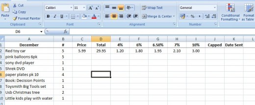
Type some headings in the first few columns at the top of the sheet, as shown here.

I have put in "December" "#" "Price" "Total" "4%" "6%" "6.5%" "7%" "10%" "Capped" and "Date Sent". For prolific sellers, you can manually add in higher percentages in new columns.
By placing the mouse at the line between the column headings (where the sheet is pale blue) the mouse pointer changes into a black perpendicular line with an east and west arrow on it. At this point you can drag the lines to widen or shrink a column, depending on the data you want to input.
I widened column A to make room for product descriptions. Also by placing the mouse on the blue 1 at the start, that whole row gets highlighted. You can then bold and/or centre the words in the whole row.

You will want to freeze that top row so that it always stays in view even when you scroll down. To do that, highlight it as shown here (by clicking in the blue box at the start of the row), then go to View ~> Freeze panes ~Freeze Top row.
Now we want to add in some products. I just made up the examples here, but you may want to write in the actual product name that you have sold. They go in the first column, under December.
I don't add a price in until it has been shipped. That way you can tell at a glance what has shipped and what hasn't. Amazon prices change quite a lot and even if you go straight to the page on Amazon to look at the price of the item sold, remember that whoever bought it, bought it the day before when the price may have been higher or lower.
So whatever product you put in first, make sure it has shipped so that you can prepare all your sums to autofill the data that comes next.
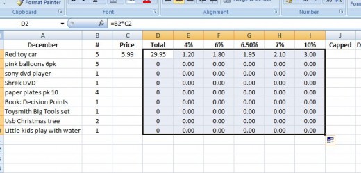
For this example, item 1 which sits in the cell A2 is a red toy car. I have sold 5 of them, and they cost $5.99 each.
In cell D2, under the heading "Total", type in =B2*C2. The equals sign tells the program, in this case Excel, that you are entering a function. Miss it out and it will not work.
If you look you are telling it to multiply the unit cost times the number of units.
The function of a cell is also viewable in the white row above, next to the fx sign. You can make changes to any or all of your functions up there, or in the cells themselves.

Now we are going along inserting all your sums.
You don't have to do this of course, as Amazon work out your percentages for you (and they always round partial numbers down!), but its handy to see at a glance how much more money you make when you reach a higher percentage.
In cell E2, under the "4%" sign, put in the formula =D2*.04
This is telling the program to give you 4% of the 29.95 the cars sold for.
It has come out at a long figure that you don't want, but that is easily fixed.
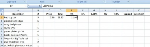
Right click on the cell and from the drop-down list that appears, choose Format Cells.
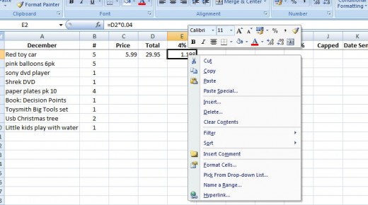
It would have been sitting on General at the very top. Click on Number, make sure it is on 2 decimal places, then click OK.
Then do the same sum in F2, G2, H2, and I2, replacing the .04 for .06, .065, .07 and finally .1.
Your spreadsheet now has its basic functions inserted.
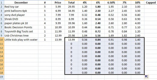
Now you want to make sure the same formula is applied to everything in those columns. I'm sure there are other ways to set that up, but all I do is highlight the cells I want repeated.
Place the cursor on the little black square at the bottom right hand side of your highlighted cells, and you will see it change from a thick white cross to a thin black cross.
At that point, grab the corner and left-button click and drag it down as many cells as you like. Your formula will input automatically in a sequential fashion. The sum in the first box will change from =D2*.04 to D3*.04, D4*.04 and so on.
Where it has no data to work with, it will return 0 until data is put in the required cells.

Now when we input our selling price for each item, the spreadsheet will automatically work out the correct figure for each cell.
What I tend to do is make a sheet for each month, and bold the column that is receiving that particular percentage. If I make enough sales to move up a percentage, I just unbold the column it was on, and re-bold the new one.
Of course excel also gives you the choice of color-coding each column to make them stand out. You can play around with the program to get things looking the way you want.
 and then click 'bold'.")
When you make more sales and want to add them in, simply highlight the bottom row and drag down as far as you want to continue the formulas down the page.

Now you will notice from this example spreadsheet that we have an electronic item in there which in Amazon.com is capped at 4%, while you may be earning 6% or more on other items. I find the easiest thing to do is to highlight all electronic items in a stand out color. I have chosen yellow.
To do this, simply go to Home ~>fill color, which has a little paint box symbol. Choose your color then click on the cell.
You can also empty the other cells in the row so you don't have to look at commission you are not earning.
In the example below I am going to show you how to add columns, though I don't usually bother. You already have your total from Amazon over on the Reports page, and chances are yours will add higher thanks to their rounding down if partial numbers.
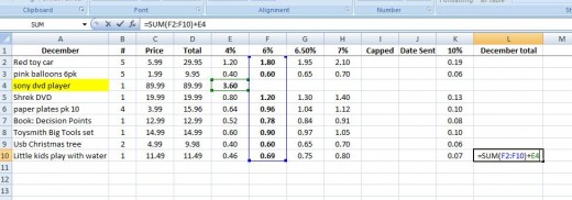
To add any column, go the the cell you want the results to show up in, and type in =sum(). Inside the brackets you want to the the first cell you want counted, and the last cell you want counted. Between the two place a colon sign.
Sop if you wanted (as in the example above) to add the column containing your 6% commission earnings, you would put in =sum(F2:F10)
But...what about the 4% you earned for selling that electronic item? Just add on the sum as I've done above - =SUM(F2:F10)+E4.I
If you wanted to know the average price of all items sold, the formula would be =average(C2:C10) or which ever column you wanted to know.
The way I have set this example page up, you would need to save it to template to re-use it every month instead of having to set up a new one.
Of course, you can also continue to use just the one sheet. replace the December heading with Product and add another column called Date.
Excel can fill each day in automatically too, just by dragging that little black box.
Have fun :)