How to Create Drop Down List in Excel 2007

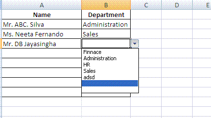
Many of us use Microsoft Excel for our day to calculations. But how many of you know how to create drop down down list Excel 2007. I am talking about something which is shown in the following figure.

• Data entry becomes easy. The data entry operator does not need to think about the spellings. They just can select from the list.

• The data is error free. No need to double check.

• This is handy in data processing too. Assume that you want to filter the employees on Department. If you have typed the departments using different formats, it would be difficult to filter them. For example if you type Department as admin in one place and administration in other place, then it Is not easy to filter the employess belonging to that department correctly using Excel filters. By using a list this problem can be overcome.

So how can you create a list in Excel? It is very easy.

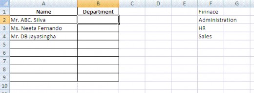
1. Type the list in somewhere in the worksheet (in my case F column).
2. Then select the cell where you want the list to appear (in this case B2) and go to Data Validation in the Data menu.

3. Select List from the Allow: drop down box in the Settings tab and for the Source select the list that you typed in the work sheet.

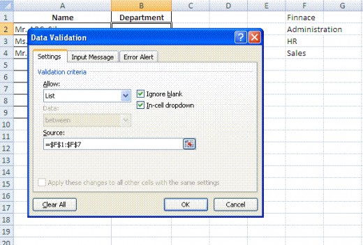
4. When you are selecting the list from the worksheet, make sure that you select few empty cells below the typed list as well. (Notice that I have selected cells F1 to F7 although I have data in cells F1 to F4 only). This will enable you adding new items to the list later without changing the formatting you applied.

5. That is it!. You are done. Now select the cell to which you applied this setting (in my case cell B2). You will see an arrow appearing to the right of the cell. When you click on it the list of departments will appear. When you select one item from the list, the cell will be occupied by that item.

6. The cool thing about this (and any formatting in Excel for that matter) is you can copy this formatting to any other cell you want. For example if you want this list to appear in all cells of column B, just copy the formatting as you copy a formula or a function. Select the cell move the cursor to the lower right corner of the cell, when you see the small cross (the cross hair) press and hold the mouse and drag down until you select all the cells. The formatting is applied to all the selected cells.

7. Just a side note; using excel macros in your worksheets and using Excel shortcut keys too will increase your efficiency, when you are working with Excel