Gun Rights: Part 2: Violent Crime: Will Reasonable Gun Control Save Lives?


FACTS
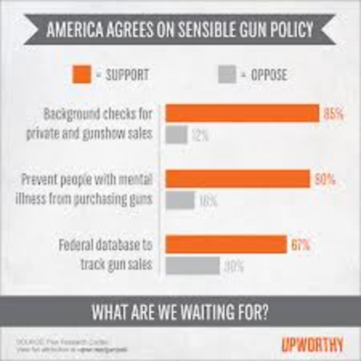
- America's Homicide Rate is almost 10 times higher than most of Europe and Canada
- America's Homicide Rate is almost 16 times lower than Russia, Venezuela, Honduras, and El Salvador
- The presence of a gun in a domestic violence situation makes it five times more likely that the woman will be killed.
- In states that require background checks on all handgun sales, 46 percent fewer women are shot to death by their intimate partners.
- Women in the U.S. are 11 times more likely to be murdered with guns than they are in any other developed nation.
Now, What About Violent Crimes?
IN PART 1, we firmly established a strong correlation between the Rate of Gun Ownership and the Rate of Death for all causes. This needed to be done first because the result is the basis of the conclusion. As you saw in the comments to Part 1, however, the concern among gun advocates is "how does the gun ownership affect violent crime?"; their contention, of course, is that it reduces it. Part 2 will take an initial, but not the only look at that question.
I pause here to note, for the record, that after working on Part 4, I found it necessary to change the titles of this series of hubs! Why? Because the problem with preconceived notions is that they are sometimes wrong. Going into this study, I felt very strongly that, like my original title suggested, "more guns leads to more violent crimes". I went so far as to end the title with "It Is As Simple As That!" Well, after doing additional analysis in Part 4 I determined "It Is NOT As Simple As That!" Consequently, I had to change to the title into a question: "Will Reasonable Gun Control Save Lives?"
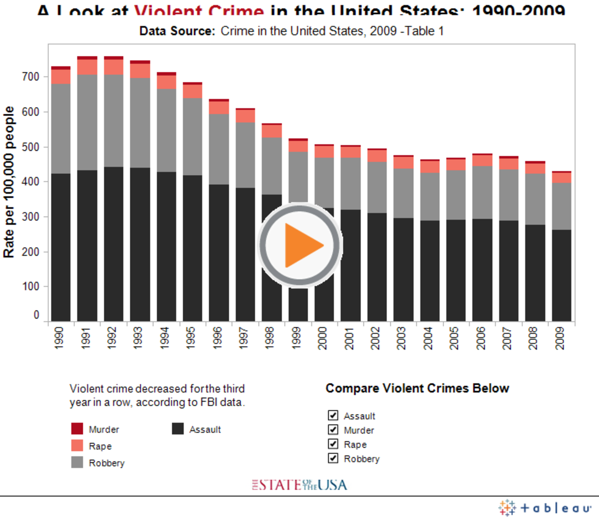
In this hub, we will consider the category of "violent" crime and its constituents: murder, aggravated assault, forcible rape, and robbery; those are the offenses which the FBI tracks as violent crimes. It is worth noting at this point that violent crime has been decreasing since 1994, except in 2006 and 2007, when there was a brief uptick. This decline coincides with the passage of the Brady Handgun Violence Prevention and Violent Crime and Law Enforcement Acts of 1994; these were the last (until 2022) major pieces of federal gun control legislation passed. Since then, the only significant action was the expiration of the assault weapon ban from the in 2004 leaving them legal to acquire and possess again. This led to an increase in mass shootings in America that has reached a crescendo in 2023 with more than 200 mass shootings in the first 165 days of the year, many of them with assault-style weapons. It took 30 years for the next piece of gun safety regulation to pass in 2022. It is called the "". The bill cleared the Senate with unanimous consent, but 190 Republicans voted against it. 1
The methodology to determine a relationship between the Rate of Gun Ownership and the Rate of Violent Crimebe is similar to the last section, just more complex. This time, however, I won't present several different scenarios as I did in Part 1 but just present the simplest reasonable formula for the "rate of gun ownership" vs. "rate of violent crime". After that, I will present the results of a multiple regression which will consider other variables. So, let's plunge on.
1 (Just a quick note - a comment was made in Part 1 that implied the US has one of the lowest violent crime rates in the world; that is not quite true. America's homicide rate, for example, is 2.8, which is 9.6 times higher than such countries as Norway, Ireland, England, France, Germany, Canada, etc. We do save some face however, for America's homicide rate is 16.3 times lower than Russia, Honduras, Venezuela, and El Salvador.)
Where Do Criminals Get There Guns?
SOURCE
| % FROM SOURCE - 2016*
| % FROM SOURCE - 1997
| % FROM SOURCE - 1991
| COMMENT
|
|---|---|---|---|---|
ILLEGAL
| 49.6$
| 39.2%
| 40.8%
| |
- Theft
| 6.4%
| |||
- Off the Street
| 43.2%
| |||
FRIENDS and FAMILIES
| 25.3%
| 39.6%
| 33.8%
| Notice shift to F & F from retail sales
|
RETAIL STORES
| 7.5%
| 8.3%
| 14.7%
| Decreased after implementation of Gun Control laws
|
PAWN SHOP
| 1.6%
| 3.8%
| 4.2%
| |
FLEA MARKET
| 0.4%
| 1.0%
| 1.3%
| |
GUN SHOWS
| 0.8%
| 0.7%
| 0.6%
| |
OTHER SOURCE
| 17.4%
| 7.4%
| 4.6%
| |
- Found at scene of crime
| 6.9%
| |||
- Brought by someone else
| 4.6%
| |||
- Other
| 5.9%
| |||
MULTIPLE SOURCES
| 2.5%
|
TABLE 1 - Source: Bureau of Justice Special Report, Nov 2001 (the last time a report like this was allowed to be published due to NRA sponsored law baring public disclosure of gun data.)
2016 - https://bjs.ojp.gov/content/pub/pdf/suficspi16.pdf
201
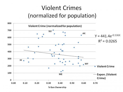
Who Brought the Shotgun
WITH NO PUN INTENDED, some of us in statistics call the above graph a "Shotgun" pattern, meaning the data points are scattered all about with no apparent pattern. Despite what looks like a downward slopping trend line superimposed on the graph, it really has no meaning. That becomes obvious when you consider the 1.2% R2 (R2 is discussed in more detail in Part 1). That low a R2 essentially implies the equation you see predicts nothing; that the average is the best estimate.
Further, if you look at another statistic concerning the constant associated with the 'X' variable, the " t-statistic", it confirms there is no definable correlation between the two variables I chose. Normally, we look for a t-statistic to be such that it shows we have a 95% level of confidence that our 'X' coefficient is not zero, but is near what the model says it is. In this case, we only have a dismal 68% level of confidence. What that means is, with this model, our best prediction, given the data we have, is the constant - 441 violent crimes per 100,000 population regardless of what the % of gun ownership is. To be honest, while I wasn't expecting that result, I am not entirely surprised.
What did startle me were the results when I looked at the separate components of violent crime using only the rate of gun ownership as a predictor. Graphs 2 - 5 provides those results.
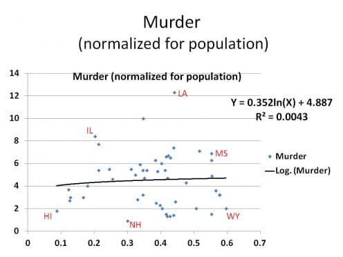
UNBELIEVABLE! WERE THE FIRST WORDS to cross my mind when I looked at Graph 2. My expectations were a noticeably upward sloping line, not a flat one. Likewise, I suspect those who advocate less gun control are equally surprised as they would expect the trend line to be sloping downward. How can the murder rate not be correlated with the rate of gun ownership, it is absolutely counterintuitive. But, there you have it, fifty data points is a reasonable number to establish a relationship if there is one.
This isn't to say that when combined with other factors gun ownership doesn't become more relevant.
Now, let's look at Rape?
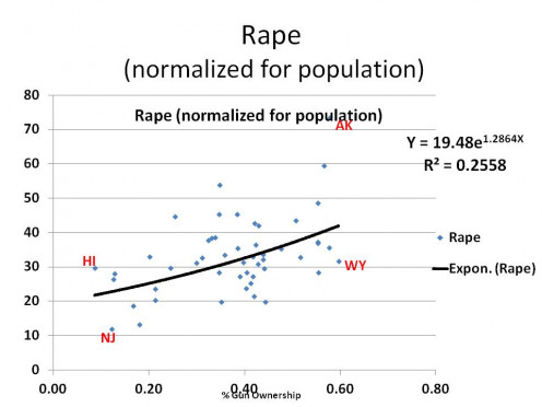
NOW THIS A BIT MORE LIKE IT. The statistics are still in the tank, meaning you cannot use the formula to generate any predictions, but the trend line is much more clear. What is interesting is rape is one of the crimes where they believe gun ownership is much more effective at preventing that specific crime. I am not going to say "apparently not", but that answer is more likely now than the opposite, based on the data.
For the moment, without further analysis, it looks like rape is independent of the rate gun ownership and averages approximately 19.48 per 100,000 population across the United States.
Now, let's look at robbery.
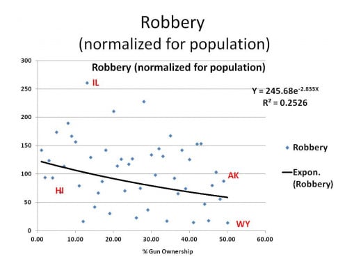
ROBBERY LOOKS LIKE THE PLOT FOR RAPE except the line appears to slope down at bit. But, like the one for Rape, looks can be deceiving for a glance at the R2 tells us our trend line is not even close to a good fit.
For the time being, the best estimate for Robberies in any state is 245.68 per 100,000 population.
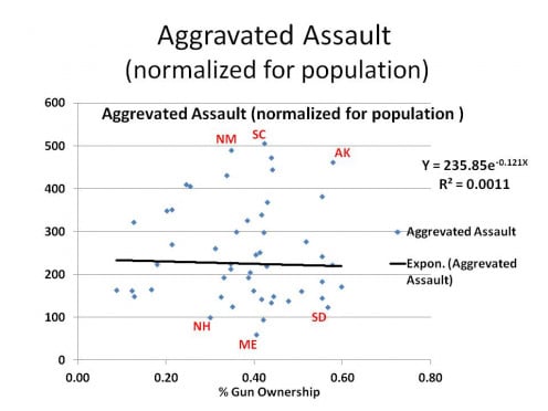
WITH AGGRAVATED ASSAULT, we are back to our shotgun pattern with no discernible trend. It is not hard to imagine, therefore, why the composite of these, Violent Crimes, also has no pattern when we consider only the Rate of Gun Ownership as a predictor of the Rate of Violent Crime.
The problem with that result is it is counterintuitive to both sides of the debate. The pro-gun lobby insists there is a negative correlation between the rate of gun ownership and the rate of violent crimes, to wit: more guns, less crime, while the pro-gun control lobby believes just the opposite. Neither would believe the results I just presented and neither do I. (In Part 4, however, I do become a believer.)
So, as any good analyst would, you look deeper into the question, you peel back the onion, so to speak. Therefore, like I did in Part 1 when I was considering Total Deaths, I will turn to looking at multiple predictors (independent variables) which, when working together, explain a correlation; and that requires multiple regression.
Since the issue is whether more guns cause more crimes, which is my hypothesis in other words, one looks for factors which are likely to influence that outcome, one way or the other. To this end, it seems to me, the density of guns in a state might work, it did in Part 1, anyway. The chart below presents one part of the result of the multiple regression.
What Graph 6 depicts is the affect the Rate of Gun Ownership has on the Rate of Violent Crime, taking into account the density of gun.
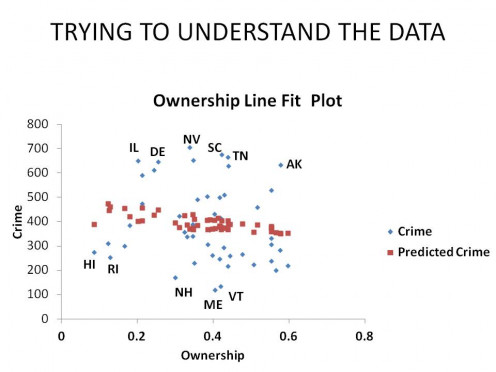
IT SHOULD BE CLEAR TO YOU BY NOW from simple observation that there is no statistical relationship between the Rate of Gun Ownership (Independent variable 1) and the Rate of Violent Crime, even when adjusted for the influence of Gun Density (independent variable 2). But, in case you don't believe me, I offer you something new, Table 1 below. It is the set of statistics one considers in judging whether a multiple regression model is reasonable or not.
Some of the numbers I look at are the probabilities highlighted in red. For the model as whole to have a 95%-level of confidence that it is producing a good result those statistics much reach certain thresholds.
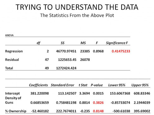
FOR ME TO EVEN CONTINUE ON with this formulation, the "Significance F" of the F-Statistic needs to be 0.05 or smaller, as does the P-Value for each of the independent variables and the intercept. By looking at the numbers highlighted in red, you can see neither the model as a whole, nor any of the variables pass this test. As a result, I need to look further.
If you look back to Graph 6, you will see I labeled data points that fell well above and below the red "prediction" data points to see what that might tell me; and it showed me something very interesting. The majority of data points across the top, which is a high violent crime rate, would be considered "Red" states, while almost all of the data points along the bottom would be considered "Blue" states.
Consequently, I used a standard analytical technique and stuck in a dummy variable into the equation where I assigned a "1" to "Red" states and a "0" to "Blue" states to see what would happen. Table 2 is the result.
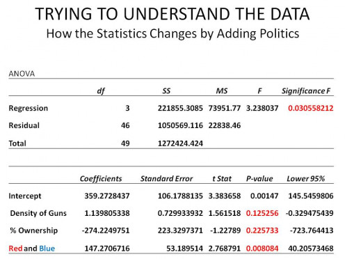
ADDING WHAT I CALL "POLITICS" INTO THE EQUATION made a dramatic improvement. Now don't anybody get to excited, on either the Right or the Left. This result doesn't mean being a conservative or being a liberal has anything to do with the Rate of Violent Crime. What it does suggest however, is that the factors underneath the reasons of why a state might be Red or Blue could have an influence. One that comes to mind is the prevalence of big metropolitan areas; an area I will dig much deeper into in a later Part.
But, for now, let's look at what we have in Table 2. The first thing we notice is the "Significance F" probability is now under 0.05 at 0.03, so the model as a whole is satisfactory in that regard. Next we can see that the intercept and the political (Red-Blue) variable have significant P-values as well, while the remaining two variables are still not significant, they got very much closer.
This means, of course, more looking. So, I turn back to my last sentence in the first paragraph about big metropolitan areas. That brings to mind one other variable that has been looked at before, population density. It seems reasonable how closely packed people are together would influence the degree they attack each other. Consequently, let's throw that into the mix and consider Table 3.
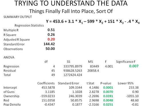
IN ONE WAY, EVERYTHING FELL INTO PLACE ... in another, it didn't. All of the statistics we have looked at so far now tell us we have a good model. Each of our variables (t-statistics, p-values) and the whole model (f-statistic, significance f) pass the less than 0.05 test; that is the good news. Why did they do that when each variable was not very good by itself? It is because of the interplay and interaction between the independent variables and how they affect the dependent variable.
For example, the rate of gun ownership seems to have a negative (reducing) influence on violent crime but the relationship is so weak as to be useless. Gun density appears to have a positive (increasing) impact on the violent crime rate, but again, by itself, has a poor correlation with the actual data. But, when the two variables are put in the same model, there is a synergistic effect that improves the predictive capability of each, but only when combined with the other.
The bad news is something I haven't mentioned in Part 2 yet, but brought up in Part 1, the "adjusted" R2. This statistic measures "goodness of fit" of the model, how well the predictions fit the data that produced the model's coefficients in the first place. We see it is .20 or 20%; meaning the independent variables explains only 20% of the variations in the dependent variable values, not a good number.
Nevertheless, I am going to ignore this problem for now because I know I can probably do better later when I do even deeper analysis. For the moment, I just want to illustrate the apparent general relationship; which, in some respects is currently bursting my bubble.
Unpacking an Equation
YOU KNOW, I NEVER UNDERSTOOD THIS STUFF when I was going to college trying to learn it, instead it took another 40 years for the material to finally sink in; talk about thick skulls! What is bothering me now is the sign on the variables X2 and X4 in the equation presented in Table 3, for my preconceived notion says it should be positive and not negative. Consequently, I need to satisfy myself that the sign is actually correct; I will tell you why in a moment.
But first, let's unpack the equation. In words, what the equation says is that the Rate of Violent Crime in terms of incidents per 100,000 population can be estimated by taking:
- 453.6 (the baseline incidents/100,000) and modifying it by adding
- 3.1 times the number of guns (X1) in the state per square mile and subtracting
- 599 times the % ownership of guns (X2) in a state and adding
- 151, if the state is Red (X3) and subtracting
- 0.4 times the number of people (X4) per square mile in a state
There are four implications from this equation:
- As the density of guns increase, so does violent crime
- If the factors which determine that more Republicans than Democrats are elected to the State Legislatures are present, then violent crimes increase 151 per 100,000 population, on average.
- The higher percentage of people who own guns in a state appears to drive down the incidents of violent crime
- As does the density of people, the higher the density, the lower the violent crime.
Neither of those negative numbers make sense to me, especially #4. Let's consider it a different way, how about the actual impact of variables X1, X2, and X4 (we know what X3 does already).
- ALASKA - Alaska is what is known as an outlier, which means its data point lies so far out of the norm, we must consider removing it from the data set; we will do that later. For now, know it contains the lowest density of guns (.73) and people (1.26), and the second highest % ownership (.578) of any State. The overall impact of those numbers is to drop the estimated violent crime rate by -193.5 to 260.1. The actual rate, however, is 632.6.
- WYOMING - It has the highest percentage of gun ownership at .597. It is also a largish, sparsely populated state with low densities, guns are 3.49/mile2 and people are 5.85/mile2. In this case, the baseline of 453.6 violent crimes/100,000 is modified by -208.1 leaving us with 245.8. Wyoming's actual rate is 219.3.
- HAWAII - Hawaii has the lowest ownership rate at .087, but pretty high densities at 18.86 and 216.8 for guns and population, respectively. The change those variables produce is -80.4, bringing the total violent crime rate down to 373.2 vs. an actual of 216.8.
- NEW JERSEY - New Jersey has the honor of having the highest density of both guns, at 140.8/mile2, and people, at 1205/mile2! Gun ownership, however, in that state is only 12.3%. That produces a -155.5 decrease in violent crimes from the baseline, leaving an estimate of 298.1. New Jersey's actual is 311.3.
I want you to notice two things.
- Wyoming, Hawaii, and New Jersey have comparable violent crime rates at 219, 217, and 311, respectively. However, they have two counter-veiling characteristics, a) Wyoming has high percentage gun ownership but low gun density, while b) Hawaii and New Jersey have low gun ownership but high gun density. That relationship is not an accident.
- Alaska, of course, breaks that mold with high gun ownership, low gun density along with a huge violent crime rate. Consider, however, that Alaska is mostly uninhabited with its small population concentrated in a small area. That effectively drives up the gun density so that you now potentially have a high gun ownership rate combined with a high gun density rate. Now the large violent crime rate is more understandable.
Summarizing Our Current State of Knowledge
FROM PART 1, WE KNOW WITH GREAT CERTAINTY, there is a strong correlation between the Rate of Gun Ownership and the Rate of Death For All Causes, primarily suicides. From Part 2, we just discovered that the Rate of Gun Ownership is weakly correlated with the Rate of Violent Crime, in general, and Murder and Robbery, specifically; there is no correlation with Rape or Aggravated Assault.
However weak that correlation appears to be at the moment, it is becoming clearer the correlation between gun ownership and violent crime is possibly negative, just as gun advocates claim. But gun ownership is not the end of the story. For the Rate of Gun Ownership to be meaningful, it must be considered in relation to, at this point of the analysis, with 1) gun density, 2) population density, and 3) state political make-up (knowing that is a substitute for other factors)
In combination, all of these factors are significant in predicting the Rate of Violent Crime, but, as important as they are, they only explain 20% of the variance in our data; not a very good model at all. Intuitively we know we are on the right track because it makes sense all of these variables are in play. The question is, what else is in play that may help explain more of the variation.
The main take-away from this hub, however, is that increasing the rate of gun ownership among law-abiding citizens, in and of itself, does not guarantee less violent crime as a whole, or of any of its components. On the other hand, from Part 1, when considering Total Deaths, there is a strong, positive (increasing) correlation between the Rate of Gun Ownership and the Rate of Total Deaths from all Causes.
With that in mind, we will next consider the Rate of Gun Ownership vs. State Gun Regulation.
Guns and Violent Crime Question
DO YOU BELIEVE THERE IS A STRONG RELATIONSHIP BETWEEN HIGH GUN OWNERSHIP RATE AND LOW VIOLENT CRIME RATE?
This content is accurate and true to the best of the author’s knowledge and is not meant to substitute for formal and individualized advice from a qualified professional.
© 2013 Scott Belford

