Basic Formatting in Excel

Formatting an Excel worksheet is like garnishing a food dish. A well garnished recipe makes it attractive and mouth-watering. Similarly, a properly formatted worksheet makes it visually fascinating and easier to understand.

decorative formatting is not always required, particularly when it’s only for our personal purpose. On the other hand if the worksheet is to be used for a large audience, a small effort in applying formatting is good gesture to convey the information we have.

Let’s understand this with the help of a simple example.

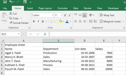
Below is a worksheet that shows Employees’ details of any arbitrary company. Keep in mind that it is the worksheet without formatting.

While below is a worksheet having formatting applied.

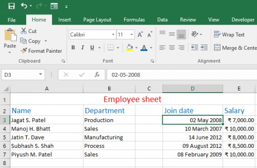
Above both worksheets contain same information, but they are represented in a different manner using formatting techniques. Worksheet with formatting looks nicer and more intuitive than one which is without formatting.

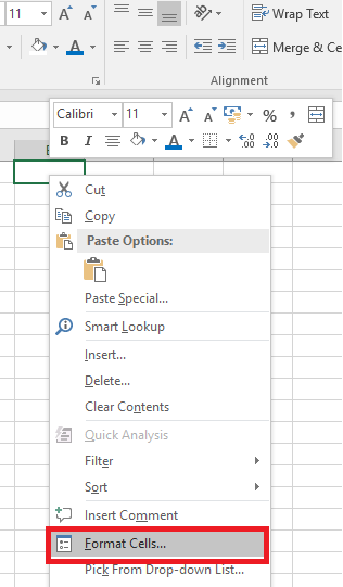
In an Excel application, format cells dialog box is a gateway of applying any kind of format except conditional format.

You can see format cells dialog box by three methods.

(i) Right click a cell or a range of cells which will open the Mini tool bar and a pop up menu. For now, forget the mini tool bar. I will discuss it later. Choose format cells option from the different options available in the pop up menu.

(ii) Press ctrl + 1 to view format cells dialog box.

(iii) Click the dialog launcher button that is seen on the bottom right corner of the font, alignment and Number sections of the Home tab.

In this hub I will discuss 3 Major sections of Excel worksheet formatting which are available on the Home tab of the Ribbon.

You can Format cell(s) by changing various font properties like type of font, size of font, font color, style of font etc. from the relevant options available in the Font section of the Home tab in the Ribbon.

You can also align the data as per your requirement and change the appearance of data by using options like merge & center, wrap the text etc. from the alignment section of the Home tab.

Excel provides number of categories to format virtually any kind of number. You can do so either from the format cells dialog box or from the Number section in the Home tab of the Ribbon.

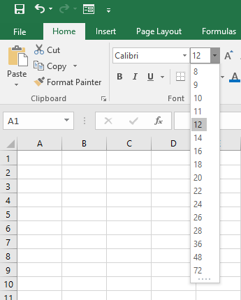
1. Changing the size of font of the selected text.It is a good practice to use different size fonts for different information like headings, subheadings and details.

   Select whichever size of font you want from the list box given in the Font tab after selecting a cell or a range of cells.

2 Changing the Type of font

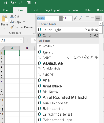
Excel’s default font type is Calibri. Other than that, it has varieties of font type that you can select from the list as shown in the figure.

3 Changing the style of font

You can apply different styles of font like bold, italic, underline or double line to the font from the options available in the font tab.

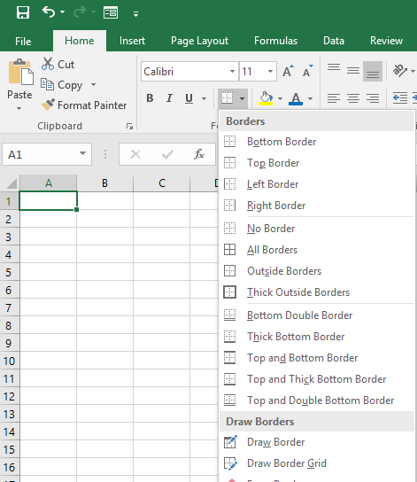
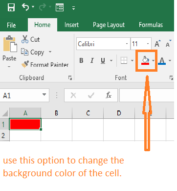
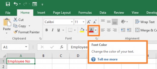
4. You can also draw borders around cell(s), change background color of the cell(s) and apply foreground color to the content of the cell(s).

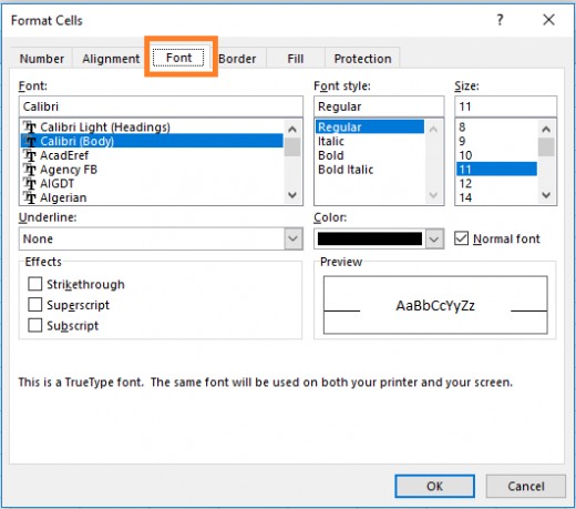
Besides the Font section, you can manipulate font properties and styles from the format cells dialog box itself as shown in the figure.

It is more advantageous to use the format cells dialog box than to use any other method as here you can see preview of your result in the preview box while changing the font properties.

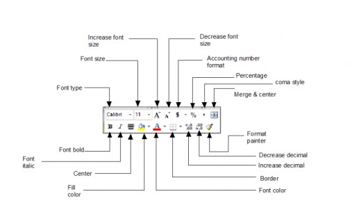
Mini tool bar is another option to deal with font properties. It is visible whenever you right click the cell(s).

Content of the cell(s) can be aligned horizontally or vertically. Default alignment type for numbers is right and it is left for text. By default all cells use bottom alignment.

You can change this default behavior from the options available in the alignment section of the Home tab. Alternatively You can use format cells dialog box for additional options.

There are primarily two categories of alignment.

(i) Horizontal alignment

(ii) Vertical alignment

(i) Horizontal alignment

Horizontal alignment type controls how content of the cell(s) are spread across the width of the cell(s). It is further divided into following sub categories.

• General- It is a default behavior. Accordingly text is aligned left and numbers are aligned right. Logical and error values are aligned in center.
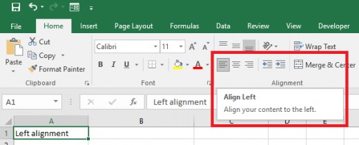
• Left- Contents of the cell(s) are aligned left side. If the width of the cell is too small to accommodate entire text, access text enters into the right hand side cell. If right hand side cell is not empty, text is shortened and partially visible.

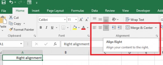
• Right- Contents of the cell(s) are aligned right side. If the cell width is too small to accommodate entire text, access text enters into left hand side cell. If left hand side cell is not empty, text is shortened and partially visible.

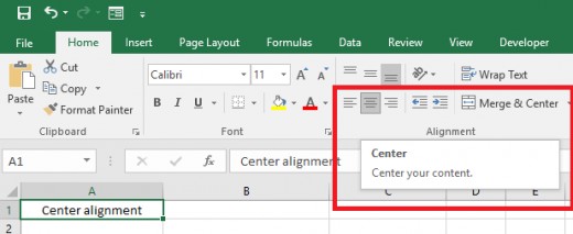
• Center- Content of the cell(s) are aligned in center. If width of the cell is too small to accommodate entire content, text enters into both sides of the cell. If nearby cells are not empty, text is shortened and partially visible.

• Fill- This option is available in the format cells dialog box. It repeats the content until end of the cell width.
• Justify- Content of the cell is justified by right and left sides i.e. it wraps the text into multiple lines because, text is too long to accommodate in a single line.
• Center across selection- This option is generally used for column headings and sub headings which when applied centers the content across more than one column.
• Distributed- Distributes or spreads the content consistently across the selected columns.

(ii) Vertical alignment

It is mostly used when the row height is set considerably more than usual. It is further divided into following sub categories.

Top- Contents of the selected cell(s) are aligned to the top side.

Center – Contents of the selected cell(s) are centered vertically.

Bottom – Contents of the selected cell(s) are aligned to the bottom side.

Justify – This option can be used along with wrap text (I’ll discus it later) and it justifies the contents of the selected cell(s) vertically.

Distributed – Distributes or spreads the content of the selected cell(s) consistently over height of the cell(s).

Wrap text- Longer texts can be accommodated in a single cell by spreading it in multiple lines using wrap text option from the alignment section.

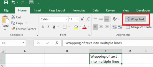
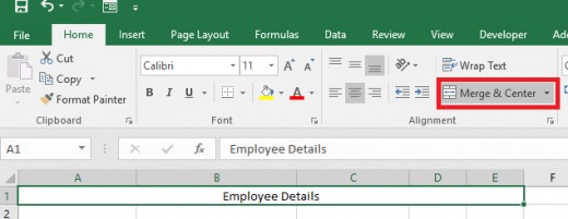
Merge & Center- This option should be used particularly when we need to keep column headings in center.

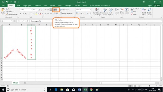
Orientation- often we need to show text at an angle for improving visual appearance of the content, this can be achieved by showing text at any angle within the range of minus 90 degree to plus 90 degree.

In some cases column width happens to be very short, at that time showing text vertically is a good option.

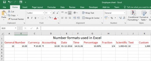
Excel provides 12 categories to format numbers.

(i) General

(ii) Number

(iii) Currency

(iv) Accounting

(v) Date

(vi) Time

(vii) Percentage

(viii) Fraction

(ix) Scientific

(x) Text

(xi) Custom

(xii) Special

(i) General- It is a default number format which is applied automatically by Excel as you type a number. General format shows the number as it is. If the width of the cell is not big enough to accommodate a whole number and the number has a decimal point then the General format rounds off that number. General format uses scientific notation for the numbers having more than 11 digits.

(ii) Number- It is particularly used for general display of numbers. It provides the facility to show large numbers with thousand separator and negative numbers in red font with or without negative sign. You can choose no. of decimal points to be applied to the number. Sample box shows the preview of your result.

(iii) Currency- It is used to display the numbers as monetary values. This format shows the symbol of a currency ahead of the number. You can choose no. of decimal places to be shown. Apart from that, you have a choice to display the negative numbers in red font with or without negative sign. Moreover, you have a freedom to select the currency symbol of country you wish form the list within the dialog box.

(iv) Accounting- Same as Currency format, it is also used for showing the numbers as monetary values. It aligns the currency symbols and decimal points of numbers in a column. Here also, you have a choice to select the no. of decimal points to be shown and whether to use a thousand separator for large numbers. The Accounting format shows zeroes as dashes and negative numbers in the parenthesis.

(v) Date- It is used to show entries in the cell(s) as Dates. The content of the cell(s) can be formatted as a date by applying different kinds of date format types. Select the type of a format in the ‘Type drop down list’ and see the result in the sample box. Click OK when you get the correct one.

(vi) Time- It is used to display content of the cell(s) as a time. Likewise date format, time can also be shown by different ways, choosing proper item from the Type drop down list. Sample box shows the result of selection of the type of time format.

(vii) Percentage- Sometimes It becomes necessary to show some numbers as percentages of a lot. This format displays the numbers as percentages by appending the % sign at the end of them.

(viii) Fraction- sometimes numbers need to be shown in fractional presentation instead of using decimal point. Fraction format exactly does so.

(ix) Scientific- Some numbers are to be shown as a scientific way. This format shows the numbers in exponential notation.

(x) Text-Data like Phone numbers, credit card numbers. Etc. are not used in calculation. So, they should be treated as text. Apply text format to the numbers that are not used for calculation purpose.

(xi) Custom- If it is not possible to show data in the cell(s) with any format types mentioned as above, a custom format should be used. Suppose we want to include a thousand separator in the number then in that case we should use custom format as per procedure mentioned below.

Select a cell having a number e.g. 25000.

Right click the cell and open format cells dialog box.

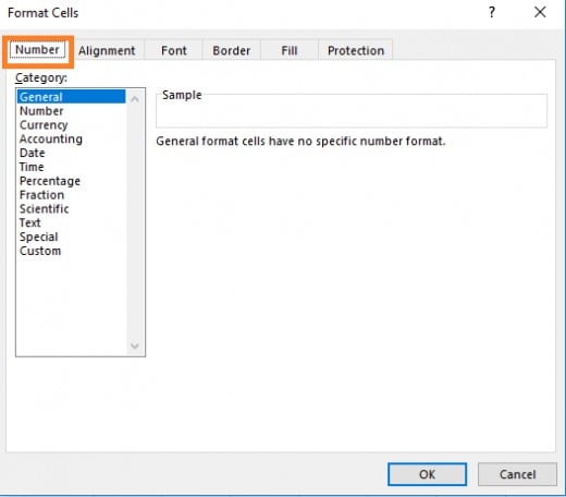
Select the number tab.

Select custom among the categories listed.

Select fourth type of custom format i.e. #,##0.

Click OK.

The number 25000 will be displayed as 25,000 in the cell.

It is a good practice to always format the Excel worksheet by using proper format techniques available within Excel application. Ribbon’s Home tab has three major sections viz. Home, Alignment and Number which are very important to understand, to make the worksheet appealing and graspable. Other than that, short cut key ctrl+1, right clicking cell(s) & choosing format cells option from the pop up menu and clicking dialog launcher button show format cells dialog box which can be used to format the cells. Mini tool bar is an additional option that helps in formatting Excel worksheet.