- HubPages»
- Technology»
- Computers & Software»
- Computer Software»
- Office Software Suites»
- Microsoft Office
Microsoft Excel - What Is A Pivot Table And How To Create One For Business Intelligence And Analysis

Why Pivot Tables?
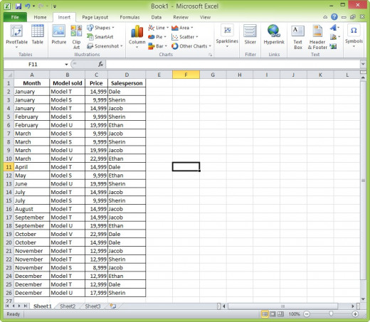
If you have been working in a corporate environment for awhile, you would most probably have come across a data table of sorts (an example on the right). This data table would tell you the relationship between an entity and various attributes/properties/variables related to that entity.
While a data table would already contain all the information you need to make sense of the relationships between the entity and it's attributes, pivot tables makes sorting through them easier (very much so!).
The most common use would be to use pivot tables to group related entities together, so that interesting variables of these entities can be summed. For example, the data table on the right shows sales of a product by month and the salesperson. You can manually eyeball for Dale's sales and add them up to see how Dale is performing as a salesperson, but a pivot table would do that for you in 2 clicks.
Read on to find out how to make your very own pivot table.
Dale sold $80,995 last year, by the way.
What Are Pivot Tables?
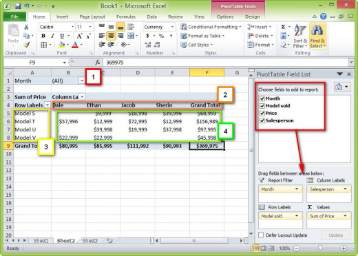
Pivot tables take data tables and turn them into smaller tables that you can easily manipulate; by 'pivoting' your pivot table according to the view you need.
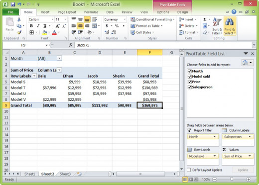
For example, the sales data table above was made into the pivot table on the right, which shows, in one small table:
- Total annual sales of each salesperson
- Total sales of each product model
One quick look at the pivot table would allow you to deduce which salesperson and product model performed the best.
How To Create Pivot Tables?
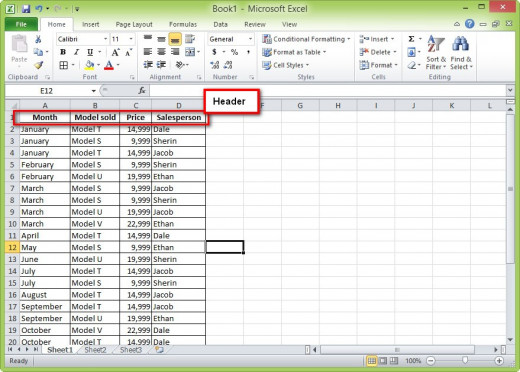
Firstly, you would need a data table that you want to analyze. Every attribute must be identified at the first column (the 'header').
Select the entire table (by using your mouse to click and hold the first cell, then dragging your mouse to the last cell) and go to the "Insert" section in the Ribbon/toolbar. If you are using Offce 2007 and above, you will see the 'Pivot Table' button as in the diagram to the right.
Click on 'Pivot Table' to see the pivot table dialogue box.
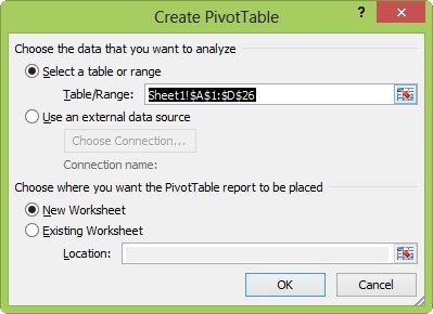
If you have already selected the entire data table, the "Select a table or range" box will already be filled in for you. So just choose if you want your pivot table to be on the same worksheet (choose "Existing Worksheet") or a new worksheet (choose "New Worksheet").
Wherever you choose to place your pivot table, you will see something like the box shown below.
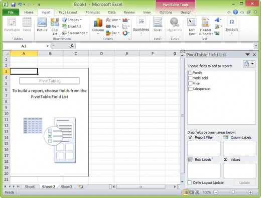
Setting Up The Pivot Table
On the right hand side, you will notice a dialogue box appears whenever you select your pivot table. This is where you manipulate what your pivot table will show. You do this by dragging the attributes you want to 'pivot' into the respective boxes:
- Report Filter - allows you to limit what data is being shown in your pivot table by any attribute
- Column Labels - determines what attributes are shown in the columns
- Row Labels - determines what attributes are shown in the rows
- Values - determines what figures are shown in the fields
Just drag-and-drop whichever attribute you want into the respective boxes.
A Pivot Table Is Created

When you're done dragging the attributes you want to analyze, your pivot table might look like the one above.
Try moving attributes around and using filters to arrive at the best pivot table to present your data.
Happy pivoting!
Want To Learn About Basic Excel Terminology?
For a list of common Excel terms and terminology, please check out my Hub here.


")


