- HubPages»
- Technology»
- Computers & Software»
- Computer Software»
- Office Software Suites»
- Microsoft Office
Using VLOOKUP in Microsoft Excel

Using VLOOKUP in Excel is a powerful way to pull data from one table into another. It stands for vertical lookup, which broken down into layman's terms, it allows you to search vertically in a table and return a specified value. As an accountant, I use VLOOKUP on a daily basis and it is an invaluable function that saves me countless amounts of time at work. It is not just limited to accountants or computer geeks, there are so many different ways to use the VLOOKUP function.
VLOOKUP Function in Excel
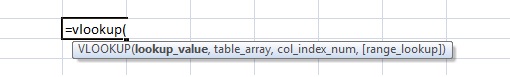
Using the VLOOKUP function is very easy once you understand how the formula works. The formula looks very technical, but it is fairly simple. The picture above lists each item that is needed to use VLOOKUP. Let us take a closer look at what each one is looking for.
Lookup Value
The Lookup Value is the value that you want to look up in the other table. It must appear exactly the same way in both tables or else it will return an error message (#N/A). The Lookup Value may either be a number or text and may be a cell reference, formula, or an actual value. In my experience, most of the time I always use a cell reference, but I have occasionally used a formula in more complex situations. This is a required part of the formula.
How would you rate yourself in Excel?
Table Array
The Table Array is simply the range of cells that you wish to search for your lookup value in. The first column contains the values that are searched for by the Lookup Value. Be sure to highlight from there over to the column that contains that data that you want to pull into the cell of your VLOOKUP formula. Also, highlight all the way down to the end of your data. I usually highlight more rows than needed, in case the table that I am pulling from eventually contains more rows of data. It is critical to anchor ($) the cell reference selection that you make here. You can easily do that by pressing the F4 key once. If you do not anchor this portion of the formula, it will not work properly when you copy the formula down because the area that you are searching will change with each row that you paste the VLOOKUP into. It is also important to remember is that this portion of the formula only works from left to right, that is, the column that you are looking up in, must be the left most column in this selection. This is also a required part of the formula.
Column Index Number
The Column Index Number is simply the number of columns over to the right that you want to go to retrieve data from. For instance, if you only want to bring back the value that you are looking up, the column number would be 1. If the data is three columns over, this would be a 3. It is important to note that you can only choose the number of columns that you highlighted or else Excel will return a #REF! error because the Column Index Number is outside of the parameters set in the Table Array. This field is also required.
Range Lookup
Range Lookup is also very simple. This value is either true, false, or it can be left blank. If you enter "true" or leave it blank, you will either return an exact match or the next closest match that is larger than what you were searching for. It is important to sort the table that you want to pull from in alphabetical or numerical order to return the correct results. Entering "false" will cause Excel to only return an exact match or an error message (#N/A). You do not have to worry about sorting when you use "false." This in my experience is the most common approach and most effective.
Limitations of Using VLOOKUP
The major limitation for using VLOOKUP is that it will only return the first match that it finds. As I mentioned above, it is important to remember when laying out your tables to make sure that the data for the array table has the column that you want to search is to the left of the field that you want to pull by using the VLOOKUP. Also, both the lookup value and the first column in the Table Array must be exactly the same. If there is an extra space at the end of one and not the other, it will cause the formula to error out.
Example of Using VLOOKUP in Excel
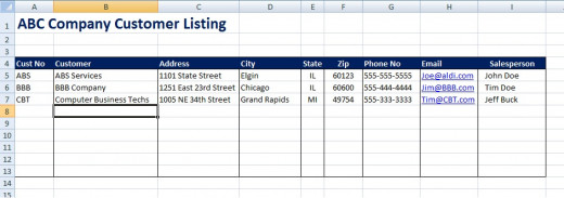
Now that you have an overview of how to use VLOOKUP in Excel, now let us look at a practical example. I created a spreadsheet with two tabs in it. The first tab, "Customer List", is a listing of customers for ABC Company as seen in the picture below:
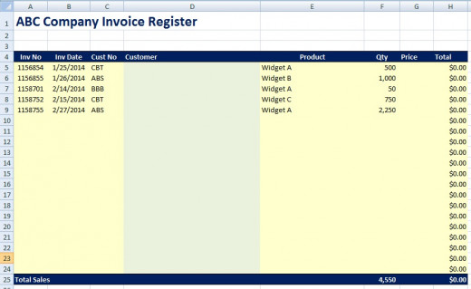
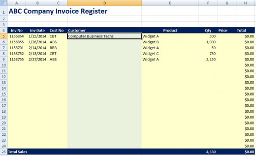
The second tab is the "Invoice Register" tab that lists all of the sales that ABC Company has made in 2014. On this tab, I will show you how to use the VLOOKUP function to pull in the name of the customer based on the "Cust No" field rather than manually typing the customer name. In my experience, it is much more efficient and accurate to pull information like this than to enter it manually because VLOOKUP eliminates any possibility of a typo when it comes to the customer name. In addition, it is much quicker once you set up the formula.
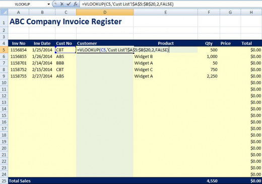
In cell D5, enter "=VLOOKUP(C5," and then click on the "Customer Listing" tab. Highlight cells A5:B20 and then hit the F4 key, which will lock the search area to those specific cells. Next, enter a "," and then a "2," because we want to return the customer name, which is in the second column. Finally, enter "false)" because we only want to return an exact match. See the example below:
Function Arguments Quick Reference Guide
Part of Formula
| Enter
| Comments
|
|---|---|---|
Lookup Value
| C5
| Click on cell C5
|
Table Array
| 'Cust List'!$A$5:$B$20
| Click on the "Customer List" tab and highlight cells A5:B20. Hit the F4 Key when finished to anchor the reference.
|
Column Index Number
| 2
| We want the Excel to look up and return the "Customer" name and that would be in the second column of the Table Array.
|
Range Lookup
| False
| Type false because we want an exact match.
|
Tip: Another way to enter a VLOOKUP Formula is to go to the "Formulas" tab in Excel and click on the small arrow below the Lookup & Reference button. A wizard window will open and ask for the above information.
Hit the enter key and you will see that the VLOOKUP has returned "Customer Business Techs" as the customer name.
Now copy the formula all the way down so that it will be ready to use as more invoices are entered. Notice how the Lookup Value changes row numbers as you scroll down. Also, notice what happens when you get to row 10.
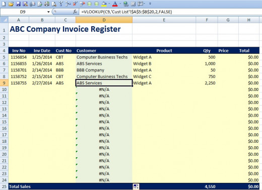
The #N/A error comes because beginning in row 10, column C is blank. This would also happen if you were to enter a "Cust No" that does not exist on the "Customer Listing" tab. There are two ways that you can add to the formula to stop this from happening. The easiest way to stop this is to add "if(iserror(" to the beginning of your VLOOKUP formula. Then hit the "End" key and enter "),""," and then copy and paste your VLOOKUP formula on to the end and add a second closing ")". The double quotation marks will cause the formula to return a blank cell if the formula errors out. You can substitute whatever you like in there including text. If you are trying to bring in a number, you may want to consider using 0 instead of the two quotation marks. See the screenshot below:
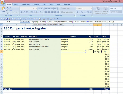
Then copy the formula down to the bottom and the #N/A error will disappear and all you will see is blank cells from row 10 to the bottom of your register.
Learning to master the VLOOKUP function will make you much more efficient when working in Excel. It is one of the most used type of formulas that I use on a regular basis. Feel free to contact me with any questions or comments.
Great Excel Resource

© 2014 Eric Cramer
Related

Analyzing Survey Data in Microsoft Excel: Coding, Inputting Data, and Creating Frequency Distributions

How to write Visual Basic code to configure a User Interface created using a UserForm in Excel 2007 and Excel 2010

Excel Time Saving Tips

How to Add a Checkbox in Excel and Automatically Generate a True or False Value in the Linked Cell

How to Format Spreadsheets in Microsoft Excel