Some Useful MATLAB Commands

MATLAB is a powerful tool which enables us to perform computationally intensive tasks. In order to use this wonderful tool efficiently and to enable yourself to harness its powers to maximum, you must know more than a newbie programmer of MATLAB knows. Most of the times, there are some commands which are overlooked or are not known at all, mainly because they appear to perform such simple tasks that could be performed by writing alternate code.

Right. These commands can be replaced by alternate code but not that easily all the time. Sometimes its really irritating to do these jobs. Using these MATLAB command greatly save our time and makes our programming simpler.

Let us get into it right away. Here is a brief description of some MATLAB commands and a few usage examples along with results. The order in which these commands appear is not significant.

fix

Usage: fix(VAR)
This command rounds the value of VAR to the nearest integer towards zero. Note the difference between this command and the simple operation of rounding numbers. Fix rounds to the nearest integer towards zero.
Example: fix(2.89) will return 2, while fix(-2.89) will return 2.
Note: The result will always be integer. If VAR is a vector or matrix the individual elements of the VAR will be changed to integers as described above.

rem

Usage: rem(X, Y)
This command returns the remainder when X is divided by Y.
Example: rem(4,3) will return 1, while rem(4,5) will return 4.

bi2de

Usage: bi2de(VAR)
This command is used to convert binary data present in VAR to its decimal equivalent. For example if VAR = [1 1;
0 1;
1 0]
bi2de(VAR) will return [ 3
2
1 ]. Note that when used this way the bi2de commands considers the right-most bit to be the most-significant bit. You can change this property by adding a second argument to the command as follows:
bi2de(VAR, ‘left-msb’). Most of the time MATLAB’s ‘reshape’ command is also used in conjunction with the bi2de command. For example if you have a vector of binary data that should be rearranged before converting it to decimal, you will use the reshape command. See reshape command here for more details.

reshape

Usage: reshape(VAR, m, n)
This command changes the size of VAR. reshape(VAR, m, n) returns the m-by-n matrix whose elements are taken column-wise from VAR. An error results if VAR does not have m*n elements.
Example: If VAR=[1 2 3 4 5 6 7 8]; reshape(VAR, 2,4) will result in
[ 1 3 5 7;
2 4 6 8]
and reshape(VAR, 4, 2) will return
[ 1 5;
2 6;
3 7;
4 8]

polyfit

Usage: polyfit(x, y, n)
Very often we are faced with the problem of mapping some data to some other numbers. Or in other words we would like to determine any relationship between these sets of data. Such problems are mostly expressed in a tabular form. For example we have the following table giving the temperature after every hour of an object used in an experiment.
Time elapsed (hours) Temperature (C)
1 80
2 130
3 138
4 140
5 150

Let us define two vectors time and temperature as follows:
time = [1 2 3 4 5]
temperature = [80 130 138 140 150]
in order to determine the relationship between time and temperature we can use the polyfit command, which by name means fitting a polynomial according to the given data. The command will be used as follows:
P = polyfit(time, temperature, 4) where 4 refers to the degree of polynomial we desire. The result will be a vector consisting of the coefficients of a polynomial P(time) i.e. you can just put the value of time in this polynomial and get the approximate temperature of the experiment at that time instant. The result in this case will be the following vector:
P = [-0.9167 15.1667 -89.0833 224.8333 -70.0000] which mathematically means P(t)= p(1)*t^4 + p(2)*t^3 + p(3)*t^2 + p(4)*t^1 + p(5)*t^0. Now just put in the value of time and you will get the temperature at that time instant. Therefore, it is evident that this command can be used to interpolation as well. i.e. you can use it to find the approximate value of temperature at those times (between 1 and 5) which are not present in the given table. An example code for this purpose is given as follows:

time=[1 2 3 4 5];
temperature=[80 130 138 140 150];
p=polyfit(time, temperature, 4);

j=1;
t=1:0.1:5;
P=p(1)*t.^4+p(2)*t.^3+p(3)*t.^2+p(4)*t.^1+p(5)*t.^0;

plot(t, P)

Well you don’t have to write that complex polynomial equation in MATLAB to evaluate a polynomial. What you need is another useful command named ‘polyval’. The above code will now be written as follows:

close all
clear all
clc

time=[1 2 3 4 5];
temperature=[80 130 138 140 150];
p=polyfit(time, temperature, 4);

j=1;
t=1:0.1:5;
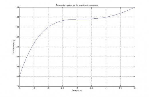
P=polyval(p,t);

plot(t, P)

The results are shown below in graphical format.

polyval

Usage: polyval(p, x)
Where p is the polynomial coefficient vector and x is the value at which we want to evaluate this polynomial. For more details please see the description of polyfit command.

floor

Usage: floor(VAR)
This command rounds the value of VAR to the nearest integer towards minus infinity. Note the difference between this command and the fix command discussed above.

abs

Usage: abs(VAR)
Abs(VAR) is the absolute value of the elements of VAR. When VAR is complex, abs(VAR) is the complex modulus (magnitude) of the elements of VAR.
Examples: abs(2.1) will return 2.1, and abs(-4.6) will return 4.6 while abs(3 + j4) will return 5.

de2bi

Usage: de2bi(VAR)
This command converts the content of VAR to their binary equivalent. The command returns a binary matrix with numbers arranged row-wise. The left most bit is the least significant bit.
Example: If VAR=[1 6 2], de2bi(VAR) will return
1     0     0
0     1     1
0     1     0

sum

Usage: sum(VAR)
S=sum(VAR) is the sum of the elements of the vector VAR. If VAR is a matrix, S is a row vector with the sum over each column. If you would like to sum along rows, use sum(VAR, 2).


Some other commands that should be reviewed:
min, max, norm, ceil.