How to Calculate Amortization Schedule in Excel

Calculation of annuities
Once you have prepared this sample, you can produce an amortization plan for different loan amounts, different interest rates, different repayment period...
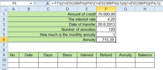
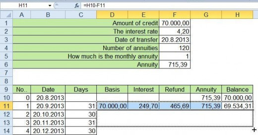
Prepare a form, such as in Fig. Note the rows and columns to copy the formula. The only information which is calculated is the annuity. The formula is quite complicated, so copy it into cell F6
= F1*((((1+(F2/(1200/F5)))^F4)*((1+(F2/(1200/F5)))-1))/(((1+(F2/(1200/F5)))^F4)-1))
Enumerated annuities
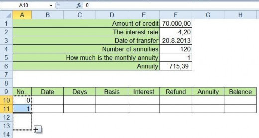
We begin with the number 0, which will be used for the initial data, starting from one, it will be numbered installment. Numbering adjust your number of installments.
The initial data
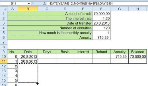
In the row below the serial number 0 is entered the date of transfer, the amount of the annuity and the initial balance equal to transfer credit. In cell B11 copy the following formula:
=DATE(YEAR(B10);MONTH(B10)+$F$5;DAY(B10))
With this formula, calculate the date of the first installment.
Calculation of the number of days
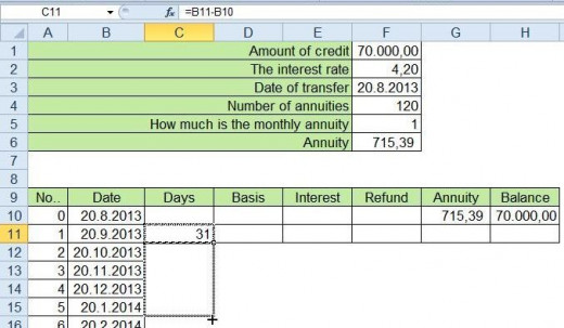
In cell C11 copy the following formula: =B11-B10
Calculate the number of days between the two dates. Copy this cell into all below it.
In the calculation of interest will take into account the principle that first day yes, last day not. Which means that the balance on the first day of reckoning into account.
The calculation basis, interest, refund, annuity and balance
The opening balance of each period is the same as the final balance from the previous period. In cell D11 copy
= H10
Interest period is calculated with the following formula:
=D11*(($F$2/IF(MOD(YEAR(B11);4)=0;36600;36500))*C11)
Copy it into the cell E11.
The amount of the loan is calculated, so to find a difference between the amount of the annuity and the interest, which were calculated for this period. In cell F11 copy the formula: =$F$6-E11
An annuity is the sum of interest and repayment of the credit. In cell G11 copy the formula: = E11 + F11
Balance is the previous balance minus the amount of repayment of principal. In cell H11 copy the formula: = H10-F11
Characterized cells from D11 to H11, and the copy of all below them.
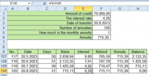
Compensation of the final balance
In the end we can conclude that we do not balance the results. This is due to rounding. Balance is leveled so that interest is calculated by subtracting repayments the amount of the annuity. In our example, we entered into a cell E130 = F6-H129.
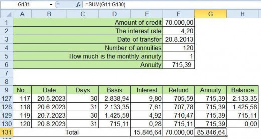
The calculation of totals
For the calculation of using the SUM function. In our case, we have
In cell E131 = SUM (E11: E130)
In the cell, F131 = SUM (F11: F130)
And in cell G131 = SUM (G11: G130)
The calculation of totals
Why are you interested in amortization schedule?
Amortization Schedule with Extra Payment
- Mortgage Calculator with Extra Payments - Mortgage Calculator
Try different options and combinations of regular or non-regular extra payments and find out how and when you can pay off your mortgage.