How to Use and Design Excel Macros - Part 4: Sample Macro Instructions

Part 3: Macro Basics

Creating a sample macro demonstrates both recording, writing, and copy-paste options to provide the user with experience designing a macro in all possible ways. These instructions also discuss defining variables, the Do While function, and the basics of manipulating graph features.

Actual process:

• Importing data to Microsoft Excel, condensing multiple columns into one, and creating a scatterplot of the values
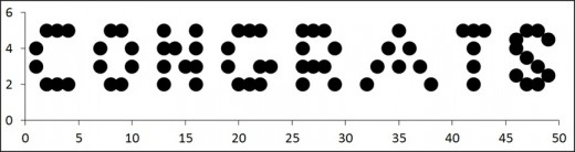
• If the instructions are followed properly, the scatterplot should spell CONGRATS

• Boolean – a type of data that can only have two values: true or false; used in conditional statements
• Function – code that stands for a specific action
• Importing – the process of bringing data into Excel from an external source
• Scatterplot – a graph of paired x- and y-values
• Variable – a character or string of characters that represents a quantity or other data

1. Open Microsoft Excel 2010. (There may be slight variations in other versions.)

2. Create a new sheet by clicking on the Insert Worksheet tab at the bottom left of the screen (alternatively Shift + F11). This will be Sheet4.

Note: The sheet is called “Sheet4” because this is how the name will appear in Excel.

3. Copy the following table, and paste it into Sheet4.

Troubleshooting: If a dark spot appears when you paste rather than the data, re-copy and paste the data table.

4. Copy the left half of the data to Sheet2, making sure to paste in the cell labeled “A1”.

5. Copy the right half of the data from Sheet4 to Sheet3, making sure to paste in the cell labeled “A1”.

6. Click the View tab at the top of the screen.

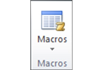
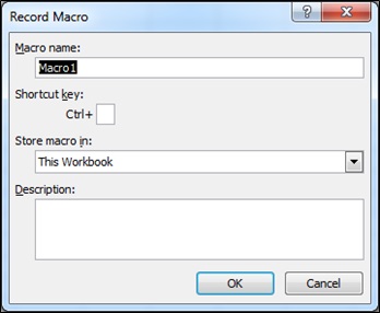
7. Select the small arrow beneath Macros (the far right icon), and click Record Macro. A dialogue box will pop up.

8. In the field labeled Macro name, type “GraphMaker”.

Note: You cannot have any spaces in a macro name. You can use an underscore ( _ ) instead if desired.

9. In the field labeled Shortcut key, type “g”. You will be able to use the keys Ctrl + g to run the macro.

10. Click OK. The Description field is optional.

11. Select Sheet2.

12. Click the arrow beneath Macros again, and choose Stop Recording.

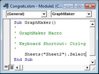
13. Select the image above Macros or View Macros. Click Edit. This will open the screen you can use to directly write a macro. It is called Microsoft Visual Basic for Applications (VBA).

You will notice that the code on the right is already written.

14. Click after the word “Select” and hit Enter on your keyboard.

15. Copy and paste the following code into the macro:

• Dim x As Integer
• Dim y As Integer
• x = 1
• y = 1
• Do While (Cells(1, x).Value <> "")
• x = x + 1
• Loop
• Do While (Cells(y, 1).Value <> "")
• y = y + 1
• Loop
• x = x - 1
• y = y - 1
• Dim a As Integer
• Dim b As Integer
• Dim c As Integer
• a = 1
• b = 2
• c = 1
• Do While (b <= x)
• Do While (a <= y)
• Cells(a, b).Cut
• Cells(y + c, 1).Select
• ActiveSheet.Paste
• a = a + 1
• c = c + 1
• Loop
• a = 1
• b = b + 1
• Loop

This code rearranges the data into a single column. First it counts the number of rows and columns. Then it goes down each column after the first and cuts and pastes each value beneath the previous in the first column.

Note: It is good practice to define your variables using the “Dim” lines, but the macro will usually function even if this is not included.

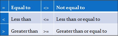
Note: The “Do While” function will continue to perform an action due to “Loop” until the condition specified is no longer met. Common Boolean expressions are listed in this table:

16. Click just before End Sub and hit Enter. Type “Sheets(“Sheet3”).Select” and then copy and paste the above code again. This time delete the “Dim” lines because the variables are already defined.

17. Again click just before End Sub and hit Enter. Copy and paste this code into the macro:

• Sheets("Sheet2").Select
• Range("A:A").Copy
• Sheets("Sheet1").Select
• Range("A1").Select
• ActiveSheet.Paste
• Sheets("Sheet3").Select
• Range("A:A").Copy
• Sheets("Sheet1").Select
• Range("B1").Select
• ActiveSheet.Paste

This pastes the columns into Sheet1.

18. Switch to the standard Excel screen by clicking the Excel icon on the taskbar at the bottom of the screen and choosing the option titled Microsoft Excel rather than Microsoft Visual Basic. (Pressing Alt + Tab will also cycle between screens.)

19. Press Ctrl + g. (Alternatively, you can click View Macros and then select Run.)

The data should be condensed into one column each and then get transferred to Sheet1.

Troubleshooting: If you made a mistake, an error message may be displayed when you attempt to run the program. If you click Debug, the line of the code that caused an issue is highlighted. You must press the Reset (blue square) button at the top of the screen before you can attempt to run the macro again. If you click End, you will have to find the issue yourself, but you will be able to run the macro again without needing to hit the Reset button.

20. Click Record Macro again. This time name the macro “Test” and assign the key “t” to it.

21. Select columns A and B. Change to the Insert tab, and click Scatter in the Chart section. Choose the first option.

22. Resize the graph by dragging the corners until it takes up the space from D7 to T20.

23. Right click on the x-axis and choose Format Axis. Select a fixed maximum of 50.

24. Right click on the data series in the graph and choose Format Data Series.

25. Change the Marker Options to Built-in circles of size 20. The scatterplot should spell out the word CONGRATS.

26. Stop Recording.

27. View and Edit the macro Test.

28. Copy the code in the macro other than the introduction and ending, and paste it at the bottom of the macro GraphMaker.

Note: You can switch back and forth between the macros by clicking on the different Modules listed on the left of the screen.

Mandatory Troubleshooting: Insert a line immediately after the scatterplot is created and type “ActiveChart.Parent.Name = "Chart 1"”. This code will ensure that the chart that was just created is the one which will be modified in later lines.

29. Switch back to the standard Excel screen.

30. Delete all data and graphs from Sheet1, Sheet2, and Sheet3.

31. Re-copy the left half of the data on Sheet4 to Sheet 2 and the right half to Sheet3.

32. Press Ctrl + g. The program should run, resulting in the creation of the graph with the word CONGRATS in large letters made of dots.

Note: The graph may have an empty title and axis labels when it is created using the macro. This can be eliminated by using another Test macro to record the deletion of these titles. (In order to make another macro with the same name, it is first necessary to delete the previous one. This can be done in the View Macros screen.) If a trendline appears as well, it can be removed in the same way.

Troubleshooting: If you have any problems, you can attempt to fix the issues using another Test macro as described in the Note above.

33. In order to save the Excel workbook so that you can use the macro again, you must click File and Save As. In the save screen, create a name for the workbook and select Excel Macro-Enabled Workbook. When the workbook is reopened, you will have to click Enable Macros to use GraphMaker and other macros.