How to use the Left and Right Function in Excel

I thought I knew a lot about Microsoft Excel until I left my first job out of college. I learned more in one year at my new job than I had learned in the previous seven years. I did not even have to take any advanced Excel training. My boss taught me many different tips and tricks in Excel including how to use macros, vlookup, auto filtering, keyboard shortcuts, and much more. I am so thankful that my boss took the time to teach me the ins and outs of Excel, which is why I love to share my Excel knowledge to try to help others. I want to share with you how to use the Left and Right functions in Excel as well as the Mid function.

The left, right, and mid functions are useful to pull text or numeric values out of a specified cell. Knowing how to use these functions can save you a lot of time. They are great tools if you are trying to automate a spreadsheet for month and year changes. They are also great for separating first and last names for mail merge purposes. Once you are comfortable using these functions, you fill find many different ways to use them.

Left Function

The Left function is great for pulling text or numeric values starting on the left side of the cell that it is pointed to. In the formula, you have to tell Excel how many spaces to pull into the current cell.

=Left([cell where you want to pull the data from],[number of characters to return])

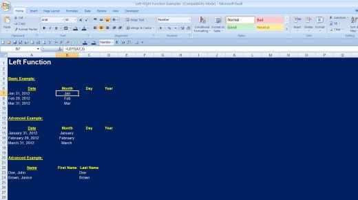
In the picture above, the “Basic Example” has a brief list of month end dates where the name of the month is abbreviated. Lets say for some reason that you need to pull the month name out of that cell. Using the Left function, the basic formula would look like this:

=Left(A7,3)

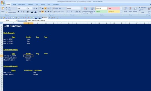
This formula will grab the first three characters in cell A7. It works great as long as all of the month abbreviations are thee characters long. Lets say that we have a list of month end dates but this time the full month is listed. We cannot use the same formula as we did with the basic example because each month has a different number of letters in it. We have to use the Find function, which looks for a specific character and returns the position of the character. For the example, we will search for the space (“ “) after the name of the month. The Find function should be included in the second half of the Left function. The formula would look like this:

=Left(A15,Find(“ “,A15))

I want to look at one more common example that is relevant if you are working with a list of names. Lets say that we have a list of names, last name first separated by a comma. This formula is almost identical, but we need to put in one additional item.

=Left(A23,Find(“,”,A23)-1)

The minus one tells Excel to find the comma and back up one space. If you did not use it, the results would be “Doe,” or “Brown,” and would not be right.

Right Function

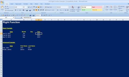
The Right function formula is similar to the Left function formula, except that it starts on the right side and moves left. If there are a set number of characters from the right side of a cell that you want to pull, the formula would look like this:

=Right(A7,4)

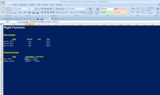
This will pull in the four-digit year. If you only want the last two digits of the year, change the formula the 4 to a 2. If you are trying to pull something out of the right side of a cell that is not a set number of characters, you will have to get fancy and use the Find function with the Len function. The Len function counts all of the characters in a cell. Under the Left function, we pulled out the last name from a list of names. Now let me show you how to pull out the first name. The formula would look like this:

=Right(A15,(Len(A15)-Find(“,”,A15)-1))

Mid Function

Out off all three functions, Mid can be the most useful because you can use it to grab things on the left, right, and middle of a cell. However it is easier to use the Left and Right functions when they are applicable. The Mid function does just what it says, it will grab characters from the middle of a cell based upon the parameters that are included in a formula. The formula starts out by defining what cell that you are looking to pull data out of, and then you will need to define the starting point where Excel should begin to return the data. This needs to be the first character that you want to return. The final part that needs to be defined is the length of the string to be returned. For instance, if the string is three digits long, the number would be 3.

=Mid(([cell where you want to pull the data from],[starting point],[length of string to return])

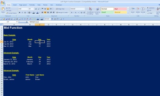
Let us return one more time to the basic example of pulling the parts for a date apart where all of the number of characters for each cell is constant. The formula would look like:

=Mid(A7,5,2)

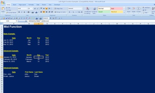
The formula will look at cell A7, and then it will go to the fifth character, and then return the fifth and sixth characters. Now let us look at a more typical use by looking at the example of having a full month plus the data and the year that we used when we looked at the Left function. This time we want to grab the day of the month from the middle of the cell. Here is what the formula will need to look like:

=Mid(A15,Find(“ “,A15)+1,2)

The “+1” is included in the formula to tell Excel to start one character to the right of what the Find function returned. The Find function does a major limitation. If there are two of the same characters in a cell, it will only find the first one. For instance, cell A15 has two spaces included in the cell. If you were to want to pull something after the second space, I would advise you to find the comma instead and put a “+2” after the Find statement.

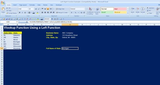
Left, Right, and Mid can be used in vlookup functions or any other kind of formula, to tell Excel what you are trying to find in a corresponding table. I choose to use Vlookup because it is one of the more advanced functions in Excel that most people will use. For this example, we are starting with a table consisting of state abbreviations and also the full name of the states. We also have an address for a company that includes a state abbreviation in the middle of a cell. Here is what the formula would look like:

=Vlookup(Mid(G5,Find(“,”,G5)+2),$A$4:$B$10,2,False)

Learning to use these Excel spreadsheet functions will help to make your life. Feel free to ask me any questions that you may have.