The Ultimate Guide to Getting Started: Google Sheets

This article is intended for the casual computer user who is marginally familiar with the basics of operating a personal computer, and can use a Web browser like Internet Explorer, Firefox, Google Chrome or similar. The examples are done on a Windows PC, but they also work on a Mac, you just need to be familiar with the basic differences between Windows and Mac operation.

It is easy to use your computer and create your own document to store any sort of information you desire! It is a great way to access information, recall it anytime you want, and a wonderful cure to the forgetfulness we often experience. This document is called a spreadsheet and can be applied to a variety of situations.

For example, my brother-in-Law collects old Coke bottles. He has an application on his iPhone that lists his complete collection, including identifying markings and condition of each bottle. When he finds a bottle that is for sale he can easily check to see if he wants to buy it.

Spreadsheets can be used in other ways too. My granddaughter used a similar program on her computer to plan her wedding, and I keep track of routine bills on my Smart Phone to avoid late payments. All these examples were done with an application called a “spreadsheet” which is normally associated with Accountants, Statisticians, and Engineers to process numerical data. But the spreadsheet has become so versatile that it is a valuable tool for keeping track of any information you want to store. Instead of writing it down in a notebook you can save it on your computer or Smart Phone.

Google has a free to use spreadsheet program that works well on your computer and your Smart Phone or Tablet. The program is called “Google Sheets”. I have provided examples of Google Sheets in this article, but the concepts are the same for any of the Spreadsheet programs on the market. Google Sheets is an online program, meaning that the program resides on the Internet and is accessed through your Web browser, this means you need an active Internet connection to work with the program on your PC. Google Sheets is a good program to use if you are not an experienced computer user because it is very forgiving and it automatically saves your work, it even has a provision for a “do over” that lets you revert back to a previous version of your file in case you really mess up.

But let us not worry about that now. The first step is to get started and I am excited to show you how!

The examples in this article were done using a Windows 10 PC and Microsoft Edge browser, you may see a slight difference if you are using a different operating system and/or browser.

This article uses “Hyperlinks” to help you navigate to sections more easily. In case you don’t already know, a “Hyperlink” is a word or phrase (called anchor text) that is usually colored different than the rest of the text, when you tap or click on the “anchor text” it takes you to the referenced location. In this case the “anchor text” will usually be the name of a Heading and the referenced location will be that Heading in this article.

Another Hyperlink use is for text describing an Internet address (URL) and the referenced location is a Web page on the Internet. Since this article is intended to be a tutorial the Internet Hyperlinks will open the referenced location in a new Tab on your browser. This allows you to stay in the article but go to the referenced Internet location by simply clicking on the new tab and return to this article by clicking on its tab. This ability to easily switch back and forth should prove useful while you work through the example in this article.

Note: You must be signed into a Google account in order to access Google Sheets, this is partly because Google saves your spreadsheet files on a “Google Drive” account on the Internet (sometimes referred to as a “Cloud” drive or simply “the Cloud”). When you create a Google account you are also set up with a Google Drive account under the same sign in name, this allows you to access your files from any computer that is connected to the internet and also share files with others if you decide to do so.

To start Google Sheets, bring up your Web Browser and type www.google.com/sheets in the address bar then press the enter key.

If you are not already signed in to a Google account you will be asked to sign in or sign up for a Google account, you will see the following screen.

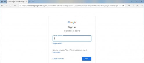
Note: If you use Gmail for your email you already have a Google account and it is assigned to your Gmail address.

If you have a Google account you can skip to "Alredy Have a Google Account" but if not click on “Create account” and you will see the following screen.

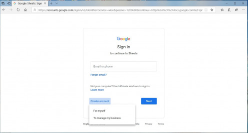
Select the “For myself” option and you will see the following screen.

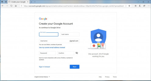
Fill in your first and last name and enter a name for your Google account or enter an existing email address and select “Use my current email address instead”.

Note: Google may provide suggestions for a Gmail account based on the information you entered.

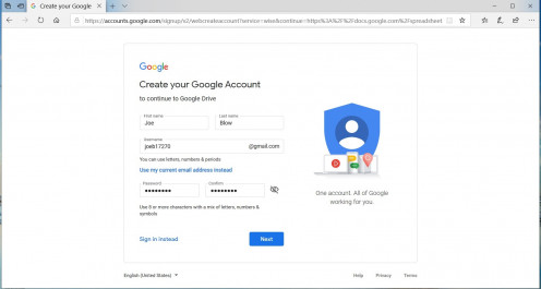
If you enter an address to use for a new account, Google will check if that name is available and, if not, will provide some suggestions for addresses that work. If the address you desire is not available, it is easiest to choose one of Googles selections.

When you enter an existing email address or accept Google creating a Gmail address for you, and provide the requested password press “Next” and you will be taken through a verification process that consists of an email sent to your email address and a phone call or text message to the phone number you provide. Once the verification process is complete you will be taken to the Sheets start page.

Please skip to "Step 2: Welcome to Google Sheets and Starting a Document".

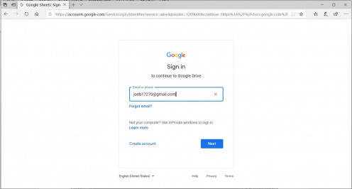
If you have one or more Google accounts, you may see the following page, or you may just see the “Sign in” page without the “Choose an account”.

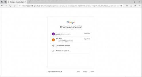
Enter or select your Google account email then click “Next”.

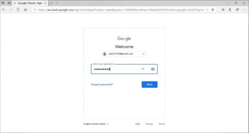
Enter your password and press “Next” then you will see the Google Sheets start page.

The first time you open Google Sheets you will see the offer To ”TAKE A TOUR”, you can take the tour if you want but, in my opinion it isn’t very informative and seems to be a waste of time. If you want to skip the tour just click on the “X” in the upper right corner of the white ”Welcome to Google Sheets” box and it will go away.

The Google Sheets welcome page offers options to start a new page or select one of the templates to help you create pre-defined spreadsheets. For this example, we will do our own thing and start a new spreadsheet.

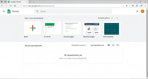
Click on the box with the colorful + to start with a blank sheet and you will see the following screen.

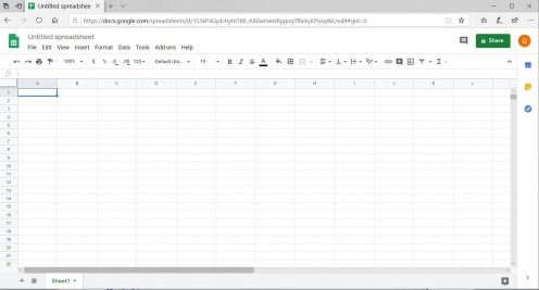
Before we go any farther you should give your spreadsheet a name to make it unique for future use. To name (or change) the name of your spreadsheet you need to click on the “Untitled spreadsheet” just to the right of the green spreadsheet icon near the upper left of the screen.

Type in the name you want for your spreadsheet, for this example let us use “EXAMPLE” for the name.

Press the "enter" key or click anywhere below the row with A B C D etc. to accept the name you have given this sheet and the screen will look like.

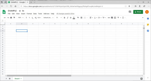
The spreadsheet consists of rows and columns of cells, each cell can hold text, numbers, or mathematical formulas. For our example we will create a “Spreadsheet” to list routine household bills, this application will only store text in the various cells. Think of it like this, our spreadsheet is like a sheet of grid paper where we write or type text in the various grids, there is no calculations involved. It will become an organized way to present our saved information.

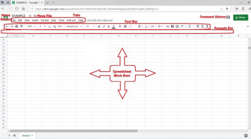
The main items on the spreadsheet screen are highlighted in Figure 15.

HOME BUTTON: The green spreadsheet icon near the upper left of the page is the “Home Button”, it takes you to the screen you saw in Figure 10.

MOVE FILE: Just to the right of the Home Button is the spreadsheet name and a “Move File button”, for this article we will be satisfied with the default file location so the move file button is not important to this project.

COMMENT HISTORY: Near the upper right edge of the page is an Icon that looks similar to the text message icon on your smart phone, this is the “View comment history” button and also is not important to this project.

SHARE: Just to the right of the Comment History button is a green button labeled “Share”, I will use this button in my next article when we share your spreadsheet with your smart phone.

TABS: Just below the spreadsheet name is a row of Tabs, clicking on a tab will show a drop-down list of tools. We will discuss those tabs that are needed for our example as we use them.

TOOL BAR: Below the tabs is the tool bar that holds the most frequently used tools for creating your spreadsheet, there are only a few tools that we need for our Example spreadsheet and we will discuss their function as we use them.

FORMULA BAR: The formula bar shows the contents of the selected cell, if the cell contains a formula the formula will be shown in the formula bar, but the selected cell will show the results of the formula.

SPREADSHEET WORK AREA: Most of the page consists of the main work area which contains cells that will hold our information.

From now on, opening and closing Google Sheets will be a much quicker process, we will discuss that a little later, for now we want to discuss our example spreadsheet. I will use my “Routine Bills” example because it will show you how easy it is to create whatever document you need to store your information.

As we said before, the spreadsheet work area consists of rows and columns of cells, the columns have letters (A, B, C, etc.) assigned to them and the rows are numbered starting at the top. Cell. A1 is the address of the cell at the first column and first row. Remember we compared the work area to a sheet of grid paper where you are free to put your information anywhere that makes sense to you.

When we think about the layout of our spreadsheet we want to start with a name or title for the project and place that at the top, on the next row we will want to assign names to each column to remind us which information we will place in each cell. We will use “Routine Bills” for the name or title, and name our columns “R”, “P”, “Company”, “Expected”, and “Due”. The columns "R" and "P" will be used to note that the bill was received and paid, "Company" is the name of the creditor, "Expected" is day the bill is expected to arrive, and "Due" is the day the bill is due.

Start by clicking cell A1 and typing “Routine Bills”, then click on Cell A2 and type “R”, next you can either click cell B2 or press the Tab key to move to the next cell (the Tab key is preferred since you don’t need to take your hands off the keyboard). Enter “P” in cell B2 and continue for the rest of the column headings.

Note: The following keys are used to navigate your spreadsheet from the keyboard

• Tab moves one cell to the right
• Shift + Tab (hold down the Shift key and press Tab) moves one cell to the left
• Home moves to the first column on the current row
• Arrow Keys move one cell in the direction of the arrow

Now I notice that some of my bills are annual, semi-annual, bi-monthly and monthly but I forgot to include a column for “Frequency”, not to worry, we can insert a column for the missing name.

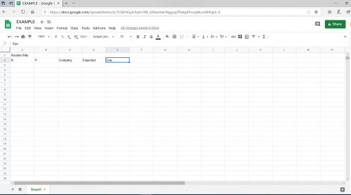
Move your mouse pointer to the letter E at the top of column E and click, notice that all of column E is selected.

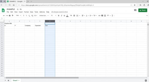
Click the “Insert” tab and notice the drop-down menu.

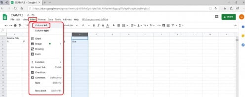
Click on “Column Left” and notice that “Due” has been moved over to column F.

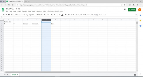
Point and click on the new blank cell E2 and type “Frequency”.

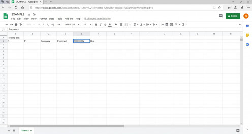
We now have a table to hold information about our routine bills but it looks a little shabby so let’s pretty it up a bit. First we pretty up the title by combining cells A1 through F1, click on cell A1 and drag (hold down the primary mouse button) the pointer over to cell F1 then release. Note that cells A1, B1, C1, D1, E1, and F1 are selected.

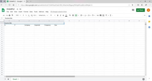
Next click the tool bar “Merge Cells” tool and the five cells become one.

Next, we want the title to be centered over our table so we select the “Horizontal align” tool, note when you click this tool a drop down appears with three choices, left, center, and right.

Click on the "center" option and notice that “Routine Bills” is now centered over your table.

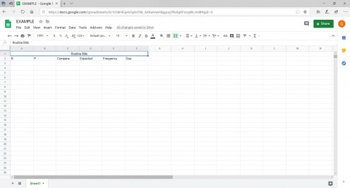
Let us center the column headings as well. Click and hold on cell A2 then drag to cell F2 and release, notice that all the headings have been selected.

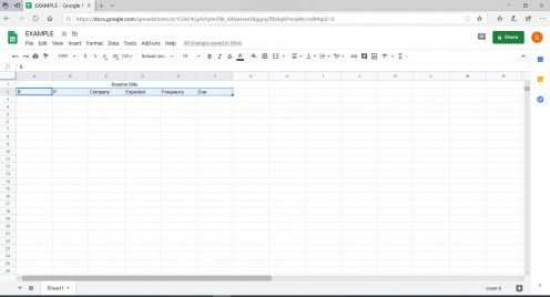
Click the “Horizontal align” tool, shown in Figure 23, and select the "center" option, notice that all your column headings are now centered.

Note: We could have selected cell A1 to F2 in Figure 24 and centered all the text at the same time.

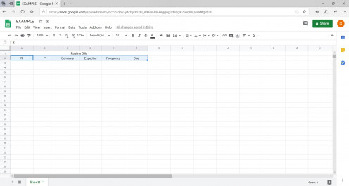
We can change the text font style, size, color, Bold and italicize to suit your taste using the text tools on the tool bar. For our example we will make all the heading text bold, click on the upper left cell in the work area then drag down to row 2 and release. Note that all the heading text is selected, this is because the upper left cell covers columns A through F and the column headings are also in Columns A through F. With all the heading text cells selected click the “B” tool on the Tool bar and notice that all the heading text is now bold.

Refer to "Figure 28" for additional tools you might find useful on the tool bar. The tools circled in GREEN are for Undo and Redo, they will back up or move forward one step for each click. The tool circled in BLUE is the Font style, when you click it a menu will drop down with other fonts you can use. The tool circled in PURPLE is the Font size, when you click it a menu will drop down with the various font sizes you can use. The tool circled in ORANGE is the italicize tool, when you click this the selected text will become italicized. The tool circled in RED is the Text color tool, when you click this tool a menu will drop down with various colors you can use for the selected text (or text in the selected cell).

Let us add Checkboxes for the "R" (received) and "P" (paid) columns. Click on cell A3 then drag to cell B3 to select the first two columns of the first row (row 3) that will contain your information, then release and observe that cells A3 and B3 are both selected. Next click on the “Insert” tab and notice the drop-down menu that appears.

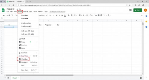
Click the “Checkbox” selection on the drop-down menu and notice that the drop-down menu disappears, and little boxes appear in A3 and B3.

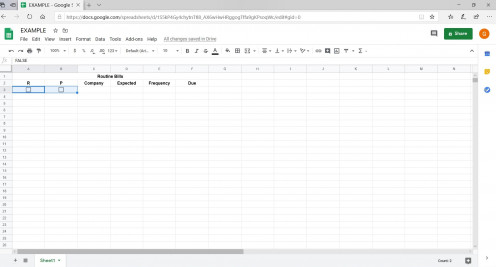
If you click on one of the boxes it turns into a box with a check mark in it (click it again and the check mark disappears) if you look at the formula bar you will see that if the box is checked it says "True" and if it is cleared it says "False", this feature will be useful in a future project. We will use the checkbox in A3 to mark when the bill arrives and the one in B3 to mark when it is paid (my bills seldom coincide with my payday, so I need to schedule their payment).

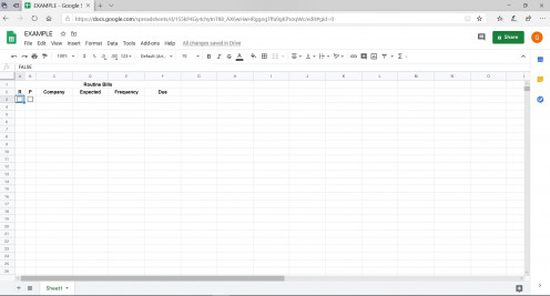
Since the Checkboxes are small, there is no need to waste so much space on their cells. We will re-size the cells to save space (this is important if we want to use our spreadsheet on a smart phone). Slide your mouse pointer across the column letters and notice that as you move from A to B the pointer turns into a two headed arrow. If you click and hold the primary mouse button you can change the width of the column to the left of the pointer by moving the mouse pointer left or right.

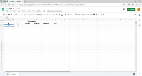
Re size columns A and B so they are just slightly wider than the check boxes.

Now we can start loading the information into our spreadsheet, I will use “American Health & Life Insurance Co.” as the first example (you can use anything you want as long as it contains several words and is fifteen or more characters long). Click on cell C3 then start typing. Notice that when the text no longer fits in the cell it spills over into the adjacent cells. We have two choices at this point, we can either make column C wider or we can format the cell so the text will wrap. I choose to make the column wider (but I will show you how to make the text wrap next).

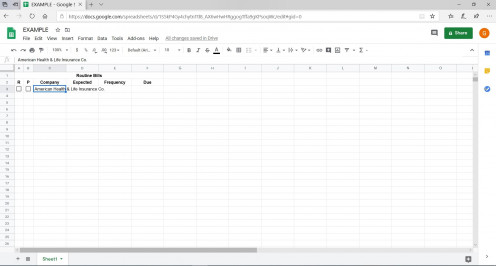
Follow the same procedure you used to change the size of cells containing checkboxes back on Figures 31 and 32 (move your mouse pointer to the intersection of columns C and D then click and drag to re size column C.)

As you enter your data you can adjust the column widths as often as you feel necessary.

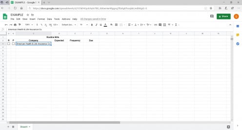
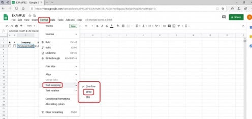
If you want to use “Word wrap” instead of adjusting the column width, you can change the formatting of the cell (or selected group of cells). To change the formatting of a cell just click that cell or range of cells (to change all cells in a column just click the heading letter for that column). Click the “Format” tab and a drop-down menu will appear, click “Text wrapping” on the menu and another menu appears. Click “Wrap” on the second menu then the menus disappear, and the selected text will wrap to fit in the cell.

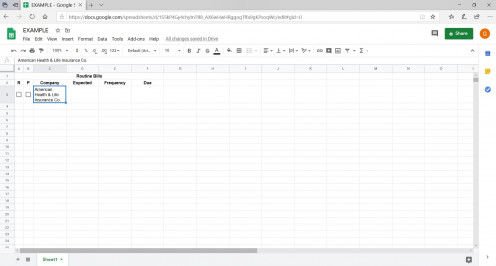
Observe that as the text in C3 wraps so it all fits in the cell width, the height of row 3 has been increased as well. If you choose “Word wrap” for all cells in a column, the row heights will adjust as necessary to accommodate the text being added.

I have added some additional entries to aid in the example and, for personal preference I choose to center the text in the “Expected”, “Frequency”, and “Due” columns. Put your mouse pointer on cell D3 then click and drag to the end of your text in cell F7 and release to select the text we want to center. Now select the “Horizontal align” tool and repeat what we did back in Figure 23. Observe that the information is now centered.

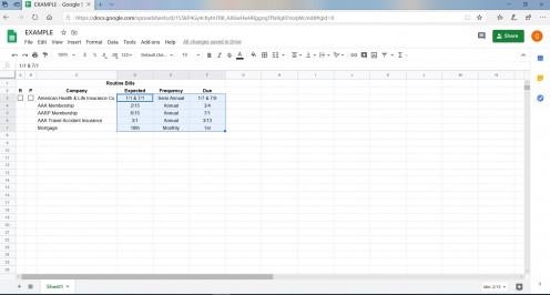
Notice that the new entries need check boxes, we will now copy the check boxes to the new lines of information. Click cell A3 and drag to cell B3 then release (it is best if you first click A3 so it shows a check, then when you click to drag the check will be cleared). Notice that cell A3 and B3 are selected and there is a little square in the lower right corner of the selection, this is called the “Fill handle”.

Move your mouse pointer to the Fill handle (little square) and (your mouse pointer changes to a +) then click and drag down to the end of the list. When you release the mouse button you will have copied Checkboxes for the rest of the rows in this example.

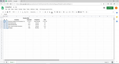
If you like the look of Boarders, you can add them using the “Borders” tool from the Tool bar. Select the section of your spreadsheet where you want the borders by pointing to and clicking on the upper left cell and dragging to the lower right cell then releasing the mouse button.

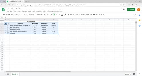
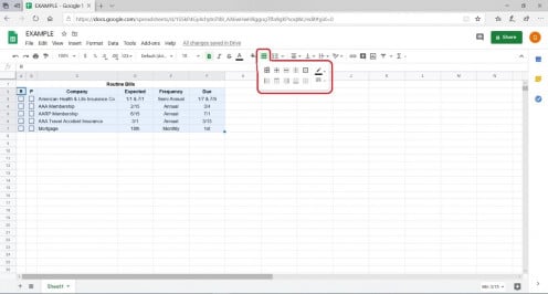
Now click on the “Borders tool” and a drop-down menu appears with various boarder options. I chose the "all borders" option, but you should try playing with different styles and colors by clicking the different buttons, remember there is an "undo" tool to get you out of trouble.

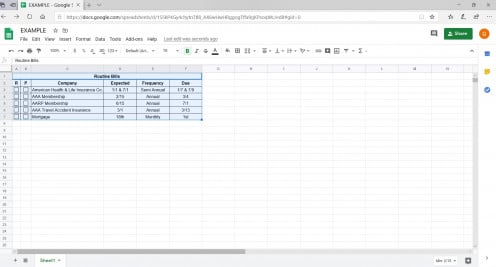
Observe that our project now has grid lines.

We need more data for our example, but I am too lazy to type more entries so instead I am just going to copy the last entry several times. Select the last entry row (move your mouse pointer to cell A7 then click and drag to cell F7 then release) then move your mouse pointer to the “Fill handle” (little square in the lower right of your selection) until it becomes a +, click and drag down to about row 30 and release. Notice that the last entry row has been copied to all the new rows.

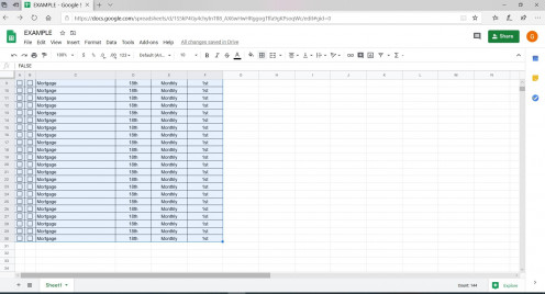
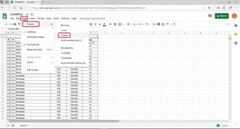
There is a problem, notice that when you drag the Fill handle down the information at the top scrolls off the screen. I no longer can see the heading information and may not be sure what each column means. Fortunately, Google sheets lets us “Freeze” rows or columns, so they say on screen while the rest of the information scrolls. To freeze the headings so they do not scroll with the data click the “View” tab then click “Freeze” on the drop-down menu then select “2 rows” on the second drop down menu.

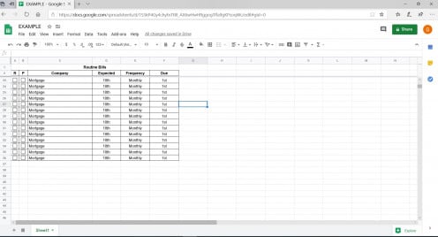
Scroll down through the data (either use your mouse wheel or the down arrow on your keyboard) and notice the headings no longer scroll with the data.

There is no need to log out of sheets, all your work is saved as you go so all you need to do is close the Sheets browser tab (or shut down your browser). When you return to Sheets, if you are still signed into your Google account you will see the Sheets welcome page. If you are not signed into Google you will see the sign in page in Figure 6, once you are signed in you will see the Sheets welcome page.

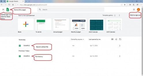
When you are on the “Home” or “Welcome” page you will see a list of all the spreadsheets you have been working on. Since we have only been working on “EXAMPLE” that is all you see, but you may see earlier versions of “EXAMPLE” listed, click on the most recent copy of “EXAMPLE” and you will return to the spreadsheet you were working on.

One more feature of Google sheets that is worth mentioning to the newcomer, is their superb “Do Over” feature. Notice just to the right of the tabs there is a comment that says “All changes saved in Drive”, this is more than just an informative note.

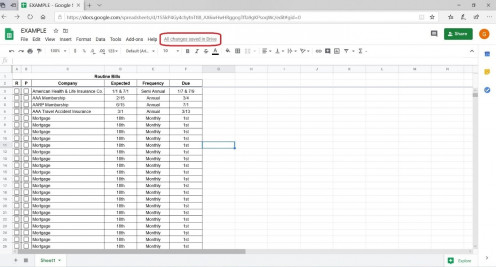
If you click on “All changes saved in Drive” the screen will change to the following:

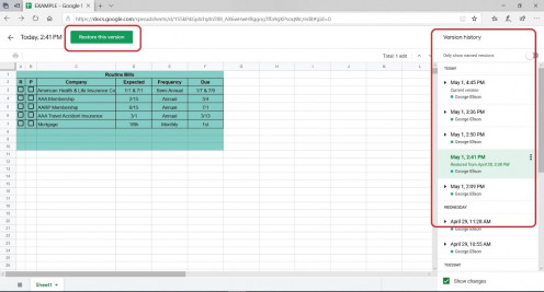
On the right you see Version history and a list of various versions of your spreadsheets. If you click on a version, it will be displayed on the screen like is shown above. Click on different versions until you see the version you want then click “Restore this version” and you are back to the version you selected. This feature can be particularly handy when you really mess up.

Last, but not least, I want to introduce you to the “Help” tab. When you click the “Help” tab you will see a drop-down menu. You can type a question or subject in the search bar (circled in green) or click “Sheets help” (circled in purple) to see a list of help topics. If you are interested in exploring Google Sheets more deeply you can try the “Training” selection.

I hope you found this article helpful and informative. Spreadsheets can be used for many things and are no longer just for mathematicians and engineers. They are for everyone! Hopefully, this article let you see how easy it is to create a spreadsheet to store anything you might desire and will lead you to experiment with your own ideas. If you are interested in using your spreadsheet on a Smartphone, please watch for my next article titled “Share Google “Docs” and “Sheets” Documents with Your Mobile Devices”.

I would also like to invite you to comment on this article, and you do not need a HubPages account to do so. I need your feedback, either good or bad, to let me know if this series is useful and if there is anything that you think should be done differently. I want to share information that helps my generation get more out of their tech devices, and I need your help to do it right.