Tutorial: How to Use VLOOKUP and HLOOKUP in Microsoft Excel Today!

Look-up functions, HLOOKUP and VLOOKUP, gather data or show information obtained from other worksheets. Using these functions is an excellent way to choose values in a large set of data. They work at displaying information by scanning columns or rows to find the particular data you are searching for in order to solve data issues.
Find the data you are looking for in a fast and easy manner by simply applying one of these formulas to your spreadsheet. A vertical lookup table displays data from columns; a horizontal lookup table displays data presented in rows.
What’s So Great about Using Look Up Functions?
- If you use the traditional way to find an exact match for your data, you may have to go through thousands of pieces of data in order to find out the information you need.
- These lookup functions are perfect when you need to search for and insert a value that is stored elsewhere in the worksheet or workbook.
- You can easily specify the rows and columns you wish to search through in order to find the lookup value.
- Using lookup functions is much faster than searching down a row or column for your information.
Have you used one of these Lookup Formulas?
If so, which formula have you used?
What is a VLOOKUP Formula?
VLOOKUP is a vertical lookup that scans a group of columns to find data that matches a specified value.
What is an HLOOKUP Formula?
HLOOKUP is a horizontal lookup that scans rows in order to find the data that matches a specific value.
Rules: These are very important. The rows or columns in a lookup formula table should be sorted by the first column or row depending on the function in order for it to work properly. In these lookup formulas, do not enter the column or row number or letter. Instead, identify the desired column and row you wish to have searched by counting the columns from the left or from the top. See the example for more details.
Fun Fact: Did you know that LOOKUP formulas were created over 20 years ago?
How to Use the VLOOKUP Formula
A VLOOKUP formula typically looks like this: =VLOOKUP(B2,Data!B2:D30,4,FALSE).
The terminology for the VLOOKUP formula is as follows: =VLOOKUP(lookup_value,table_array,row_index_num,range_lookup).
It may seem trying at first, but once you practice, get the hang of using it, and use it frequently, you will find that this formula will make your life easier. This is a brief overview of what this formula is all about, but an example will be shown later in this article that will help you easily understand how to use it.
Now that you have become familiar with the terminology of this function, learn the details of the formula in this table.
=VLOOKUP
Part
| Definition
|
|---|---|
Lookup_value
| This is the value searched for in the table array
|
Table_array
| This is the range of information the formula searches for to find your data
|
Col_index_num
| This is the column number in your defined range of cells that contains the value you wish to have returned to you
|
Range_lookup
| TRUE or blank provides you with an approximate match and FALSE provides you with an exact match
|
Note: Do not put spaces between any items after the equal sign. It will throw off the formula, and you will not receive your desired result.
How to Use the HLOOKUP Formula
An HLOOKUP formula typically looks like this: =HLOOKUP(J2,SumDataInfo!C2:R80,8,FALSE).
The terminology for the HLOOKUP formula is as follows: =HLOOKUP(lookup_value,table_array,col_index_num,range_lookup).
It may seem trying at first, but once you practice, get the hang of using it, and use it frequently, you will find that this formula will make your life easier.
Since tables or arrays of data are not typically designed in a horizontal manner, VLOOKUP is much more commonly used than HLOOKUP. You may wish to focus on learning how to use the VLOOKUP formula first and foremost.
The HLOOKUP formula, when needed, will come naturally after mastering the VLOOKUP formula. However, if you wish to learn both today, keep reading! This is a brief overview of what the HLOOKUP formula is like, but an example will be illustrated later in this article that will help you understand how to use it with ease and comfort.
Now that you have become familiar with the terminology of the HLOOKUP formula, learn the details in the following table.
=HLOOKUP
Part
| Definition
|
|---|---|
Lookup_value
| This is the value searched for in the table array
|
Table_array
| This is the range of cells the formula searches for to find your data
|
row_index_num
| This is the row number in your defined array that contains the value you wish to have returned to you
|
Range_lookup
| TRUE or blank provides you with an approximate match and FALSE provides you with an exact match
|
Note: Do not put spaces between any items after the equal sign. It will throw off the formula, and you will not receive your desired result.
VLOOKUP Formula
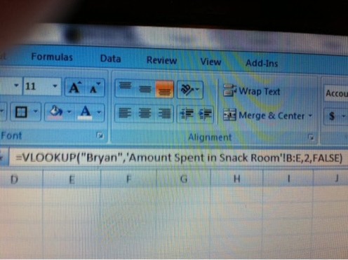
VLOOKUP Example
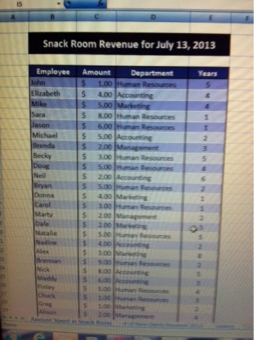
Example on How to Use the Lookup Formulas
Okay, so maybe I am picking on my man, Bryan, in this example, but here it goes.
VLOOKUP
The first example is one on VLOOKUP. This table is set up to show how much money was spent in the break or snack room of the office on July 13, 2013 per employee.
We will look at the following parts to the formula: (1) the lookup value, (2) the table array, (3) the column index number, and (4) the range lookup.
So, in my little example:
(1) I want to know how much Bryan spent in the break room on July 13, 2013; my value is “Bryan” (Note: Since it is text, it belongs in quotation marks with no spaces.),
(2) I am putting my formula in a separate worksheet (in the same workbook) so I am referencing the table Amount Spent in Snack Room in this manner: ‘Amount Spent in Snack Room’! and then with NO spaces I am adding the table array of B:E, meaning go through all the cells in columns B through E,
(3) As you can see in the picture, the “Amount” spent in the snack room is the column after the name. This means my value (Bryan – the name) is equal to 1 and what I want ($5.00 – the Amount) is equal to 2, so the number 2 is entered for this value, and
(4) Bryan is the only employee listed with that name, so his name will only appear once on this list in the way it was organized. Therefore, I want an exact match, so FALSE is entered as the range lookup.
HLOOKUP Example
HLOOKUP
The second example is for HLOOKUP.
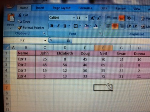
This table tells me per quarter how many new clients each employee retained. I want to know how many clients Bryan gained in the third quarter of 2013.
We will look at the following parts to the formula: (1) the lookup value, (2) the table array, (3) the row index number, and (4) the range lookup.
So, in the following example:
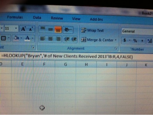
(1) I want to know how many clients Bryan gained for the company in the third quarter in 2013; my value is “Bryan” (Note: Since it is text, it belongs in quotation marks with no spaces.),
(2) I am putting my formula in a separate worksheet (in the same workbook) so I am referencing the table # of New Clients Received 2013 in this way: ‘# of New Clients Received 2013’! following it with no spaces I am adding the table array of B:R, meaning go through all the cells in rows B through R,
(3) As you can see in the picture, the “Qtr 3” clients gained in 2013 is three rows after the name. This means my value (Bryan – the name) is equal to 1 and what I want (32 – the number of clients gained by Bryan in Qtr 3) is equal to 4, so the number 4 is entered for this value, and
(4) Bryan is the only employee listed with that name, so his name will only appear once on this list in the way it was organized. Therefore, I want an exact match, so FALSE is entered as the range lookup.
HLOOKUP Formula
An Introduction to VLOOKUP For Beginners
Conclusion
These formulas or functions will allow you to search through one or more columns or rows of data for a specific value. Then, you can have the specific value returned in your desired formula cell, preventing you from searching through too much data.
Instead of you having to search through thousands of rows or columns of data, a magic formula will display the information you need that resides within another set of data. This data could be in another worksheet or in another array of data.
Save yourself time by learning new ways to do things in Excel, and you know what they say? Saving time means saving money!
Want to Learn More? Learn How to Make a Pivot Table!
- Tutorial: How to Create a Simple Pivot Table in Microsoft Excel
This tutorial walks you through step by step the way in which to create and edit an Excel pivot table. Pivot tables organize data, allow you to view trends, and help you make informed decisions.
Learn Excel Short-Cuts That Will Save You Time and Impress Others
- Outshine Coworkers with these Excel Tricks: Not Normal Shortcuts
This article will provide you with seven easy Microsoft Excel lessons with outlets to speed your typing! These secret tips and tricks are not typically taught or shared so enjoy!
Disclaimer
Pictures: The pictures used in this article were taken by Michele Jones.
Videos: The provided videos were from You Tube.
HubPages: Feel free to ask a direct question regarding this article in the comment section. If you found this article to be useful or interesting, please:
- Rate it
- Share it
- Leave a Comment or Question.
Thanks for stopping by!


