How to calculate XIRR using Microsoft Excel to know how much your loan costs
To be honest I don’t suggest buying a car through a loan for many reasons, so I am going today to explain just one reason, & I think it will be enough for you to think again before buying a car using facilities.
At least when you decide to do that, you should know what you actually pay.
Example
If you want to buy a $10000 car, and you don’t have cash, you will start to look for a financial facility.
Finally, you find the chance for a loan charging you just 8% yearly. The employee will tell you the following:
1- We just charge 8% yearly, so $10000*8% = $800 suppose you will pay in full within two years so $800*2= $1600.
2- As is a loan you just have to pay $500 as other fees as it is not cash sales, & he will start give you a list of reasons.
3- So you have to pay just $1600+$500= $2100 more during two years.
4- First payment should just 10% of the cash cost $10000*10%= $1000
5- Monthly installment will be just $442.
6- Initial payment will be (10% the cost + other fees+ one installment) =($1000+$500+$442) = $1942. (Just 19.42% of the cash cost).
7- Look how much you are lucky, now you have a car loan costs you just 8%.
Q: Are you happy?
A: As accountant, I am not happy at all, because easily I will take his offer and go to my office, I will open Microsoft office Excel & use a very simple function (XIRR) to find that this loan will cost me 27.24% a year.
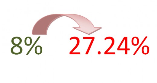

Why the rate has been changed from 8% to 27.24%?!!
1- Because when you received the car you directly paid 10% of cash value of the car, so the loan amount is $9000 and not $10000.
2- You paid $500 more as other fees.
3- You started to pay first payment on the same day you received the car.
4- You are paying monthly installment, so the loan amount is reducing month by month (You are not taking the car & pay the loan and its interest after 2 years in bulk).
Microsoft Excel Books
Excel Sheet
How do I use XIRR formula in MS Excel ?
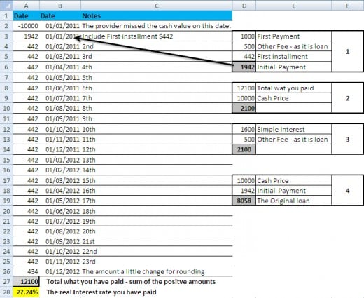
Suppose you are the bank or the service provider so you missed $10000 cash when you delivered the car, let us say on 1-1-2011, to your customer so this amount is negative.
But the amount you received starting from 1-1-2011 all are positive.
A- In first column A enter:
1. In cell A1 enter the word (Amount).
2. In Cell A2 enter -10000 (minus ten thousand) the value you missed on 1-1-2011.
3. In Cell A3 enter 442 the value you received on 1-1-2011.
4. So on for all installment till A26 which contain the last amount you should pay.
B- In Second column B enter the appropriate date beside each amount till B26 which has the date of 24th installment.
C- In cell A27 enter this “=SUM(A3:A26)” so you get the total of the amounts they have received from you.
D- In cell A28 enter “=XIRR(A2:A26,B2:B26)” (this is the Syntax = XIRR(values,dates) so you get 27.24% as a result.
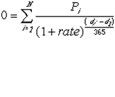
Excel will use this formula
Learn Microsoft Excel
You should do same when you get an offer, anyway I will be ready to help calculate the rate for you, if you give all the needed data (cash cost, Initial payment amount, the dates, the monthly installment).
Always calculate before you buy.
Note:this can work for any kind of loans having installments.
Hope it helps.


